Section 13: Hydrograph Method
A hydrograph represents runoff as it varies over time at a particular location within the watershed. The area integrated under the hydrograph represents the volume of runoff.
Estimation of a runoff hydrograph, as opposed to the peak rate of runoff, is necessary for watersheds with complex runoff characteristics. The hydrograph method also should be used when storage must be evaluated, as it accounts explicitly for volume and timing of runoff. The hydrograph method has no drainage area size limitation.
shows that in cases for which a statistical distribution cannot be fitted and a regression equation will not predict adequately the design flow, some sort of empirical or conceptual rainfall-runoff model can be used to predict the design flow. Such application is founded on the principle that the
of the computed runoff peak or volume is the same as the AEP of the rainfall used as input to (the boundary condition for) the model.
The hydrograph method is applicable for watersheds in which t
c
is longer than the duration of peak rainfall intensity of the design storm. Precipitation applied to the watershed model is uniform spatially, but varies with time. The hydrograph method accounts for losses (soil infiltration for example) and transforms the remaining (excess) rainfall into a runoff hydrograph at the outlet of the watershed. Figure 4-10 shows the different components that must be represented to simulate the complete response of a watershed.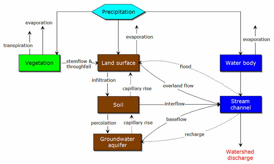
Figure 4-10. Components of the hydrograph method
Because the resulting runoff hydrograph is a time series of flow values, the method provides a peak flow value as well as volume of runoff. This makes the method suitable for design problems requiring runoff volume as a design parameter.
Successful application of the hydrograph method requires the designer to:
- Define the temporal and spatial distribution of the desired design storm.
- Specify appropriate loss model parameters to compute the amount of precipitation lost to other processes, such as infiltration, and does not run off the watershed.
- Specify appropriate parameters to compute runoff hydrograph resulting from excess (not lost) precipitation.
- If necessary for the application, specify appropriate parameters to compute the lagged and attenuated hydrograph at downstream locations.
Basic steps to developing and applying a rainfall-runoff model for predicting the required design flow are illustrated in Figure 4-11. These steps are described in more detail below.
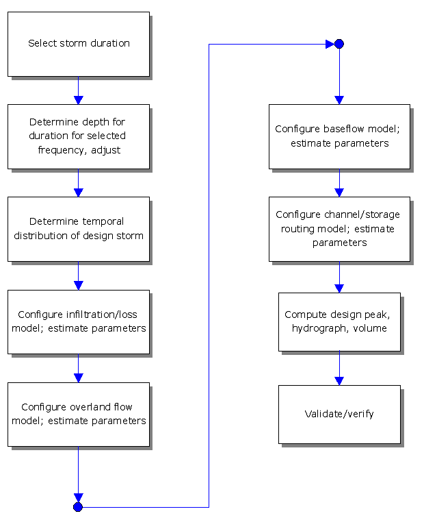
Figure 4-11. Steps in developing and applying the hydrograph method
Watershed Subdivision
The method is also applicable to complex watersheds, in which runoff hydrographs for multiple subbasins are computed, then routed to a common point and combined to yield the total runoff hydrograph at that location.
TxDOT research on undeveloped watersheds (0-5822-01-2) has indicated that there is little justification for subdividing a watershed for the purpose of improving model accuracy. In general, subdivision had little or no impact on runoff volume for the following reasons:
- In general, subdivision of watersheds for modeling results in no more than modest improvements in prediction of peak discharge. Improvements generally are not observed with more than about five to seven subdivisions;
- Watershed subdivision multiplies the number of sub-process model parameters required to model watershed response and introduces the requirement to route flows through the watershed drainage network. Discrimination of parameters between sub-watersheds is difficult to justify from a technical perspective;
- The introduction of watershed subdivisions requires hydrologic (or hydraulic) routing for movement of sub-watershed discharges toward the watershed outlet. The routing sub-process model requires estimates of additional parameters that are subject to uncertainty;
- The dependence of computed hydrographs on internal routing became more apparent as the number of subdivisions increased; and
- Application of distributed modeling, as currently implemented in HEC-HMS, was difficult and time consuming. It is unclear what technical advantage is gained by application of this modeling approach in an uncalibrated mode, given the level of effort required to develop the models.
There are circumstances in which watershed subdivision is appropriate. If one of the sub-watersheds is distinctly different than the other components of the watershed, and if the drainage of that sub-watershed is a significant fraction of the whole (20-50%), then a subdivision might be appropriate. Specific examples of an appropriate application of watershed subdivision would be:
- the presence of a reservoir on a tributary stream,
- a significant difference in the level of urbanization of one component of a watershed, or
- a substantial difference in physical characteristics (main channel slope, overland flow slope, loss characteristics, and so forth).
- unique storm depths are appropriate for the different subbasin areas.
- computed hydrographs are needed at more than one location.
Design Storm Development
A design storm is a precipitation pattern or intensity value defined for design of drainage facilities. Design storms are either based on historical precipitation data or rainfall characteristics in the project area or region. Application of design storms ranges from point precipitation for calculation of peak flows using the rational method to storm hyetographs as input for rainfall-runoff analysis in the hydrograph method. The fundamental assumption using design storms is that precipitation of an
yields runoff of the same AEP.
Selection of Storm Duration
Selecting storm duration is the first step in design storm modeling. The appropriate storm duration for stormwater runoff calculations is dependent on the drainage area’s hydrologic response. The selected storm duration should be sufficiently long that the entire drainage area contributes to discharge at the point of interest. Storm duration is defined in terms of time of concentration (t
c
), which is the time it takes for runoff to travel from the hydraulically most distant point of the watershed to a point of interest within the watershed.For complete drainage of the area, time for overland flow, channel flow, and storage must be considered. Typically for hydrograph computations the storm duration should be four or five times the
. Longer duration of storm will not increase the peak discharge substantially, but will contribute greater volume of runoff.
Commonly, a storm duration of 24 hours is used. However the 24-hour storm duration should not be used blindly. Runoff from longer and shorter storms should be computed to demonstrate the sensitivity of the design choices.
For TxDOT, the 24-hour storm should be used as a starting point for analysis. However, if the analysis results appear inconsistent with expectations, site performance, or experience, an alternative storm duration should be considered. In that case, the designer should consult the Design Division Hydraulics Branch for advice.
Storm Depth: Depth-Duration-Frequency (DDF) Relationships
Once the storm duration is selected, the next step is to determine the rainfall depth or intensity of that duration for the selected AEP.
Depth-Duration-Frequency (DDF) data at each project location is available from the 2018 NOAA Atlas 14 data and accessible through NOAA's Precipitation Frequency Data Server (
). The PFDS is a point-and-click interface developed to deliver NOAA Atlas 14 precipitation frequency estimates and associated information. The PFDS values have been developed on a 300m grid system. For larger watersheds, engineers will need to use judgment in selecting a reasonable point to establish depth values. Consideration should be taken with respect to varying depths across the watershed. The location of the selected depth values and a brief explanation should be reported in the drainage report or plans. Estimates and their confidence intervals can be displayed directly as tables or graphs. From drop-down options on the website, appropriate data type (depth or intensity) and timeseries type (partial duration or annual maximum) should be selected prior to selecting the location. Annual maximum should be selected as the time series for most analyses. Certain municipalities may have a stated preference for use of partial duration and if so, to minimize model differences, that time series type may be used.
The AEPs represented are 1/2, 1/5, 1/10, 1/25, 1/50, 1/100, 1/200, 1/500, 1/1000 (2-, 5-, 10-, 25-, 50-, 100-, 200-, 500-, and 1000- years). The storm durations represented are 5, 10, 15,30 and 60 minutes; 2, 3, 6, and 12 hours; and 1, 2, 3, 4, 7, 10, 20, 30, 45 and 60 days. The depth or intensity for the strom with an Average Recurrence Interval (ARI) of one year is provided with partial duration series.
The prior data source for rainfall was the
(TxDOT 5-1301-01-1, 2004). This was an extension of a 1998 USGS
study and an update of
(Hershfield 1961),
(Miller 1964), and
(Frederick et al. 1977). All these prior precipitation reports are considered superseded for Texas with the 2018 NOAA Atlas 14 data.
Intensity-Duration-Frequency Relationships
While hydrograph methods require both rainfall depth and temporal distribution, the rational method requires only intensity. The rainfall intensity (I) is the average rainfall rate in inches/hour for a specific rainfall duration and a selected frequency. For drainage areas in Texas, rainfall intensity may be computed by:
- UsingDepth-Duration-Frequency (DDF) tabular data/graphs for Texas from the NOAA Precipitation Frequency Data Server ( )to obtain the precipitation depth for a given frequency.
- Converting the precipitation depth to a precipitation intensity by dividing the depth by the storm duration. The precipitationintensityis measured in inches/hour.
For example, if the 100-year, 6-hour depth is 3.2 inches, the
average
precipitation intensity over those 6 hours
equals 3.2 inches/6 hours = 0.53 inches/hour. However, the IDF relationships are available from the PFDS server and may be obtained directly without performing this conversion.
Areal Depth Adjustment
When estimating runoff due to a rainfall event, a uniform areal distribution of rainfall over the watershed is assumed. However, for intense storms, uniform rainfall is unlikely. Rather, rainfall varies across the drainage area. To account for this variation, an areal adjustment is made to convert point depths to an average areal depth. For drainage areas smaller than 10 square miles, the areal adjustment is negligible. For larger areas, point rainfall depths and intensities must be adjusted. Two methods are presented here for use in design of drainage facilities: the first is by the US Weather Bureau and the second is by
.
US Weather Bureau Areal Depth Adjustment
The US Weather Bureau (1958) developed Figure 4-11 from an annual series of rain gauge networks. It shows the percentage of point depths that should be used to yield average areal depths.
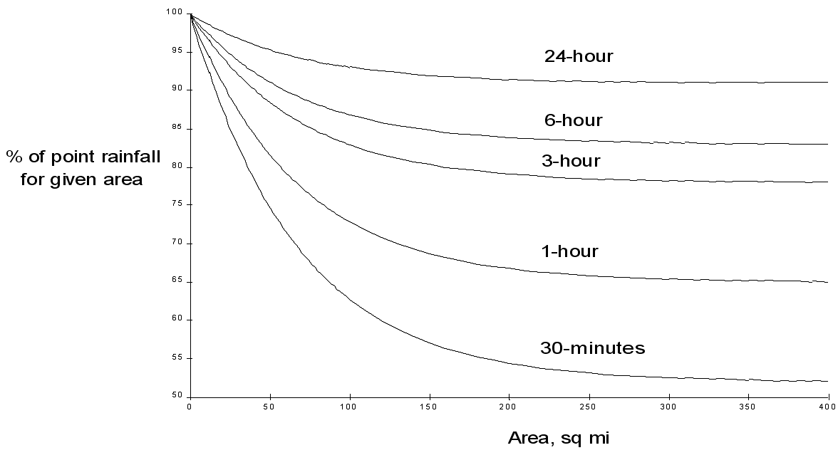
Figure 4-12. Depth area adjustment (US Weather Bureau 1958)
USGS Areal-Reduction Factors for the Precipitation of the 1-Day Design Storm in Texas
Areal reduction factors (ARFs) specific for Texas for a 1-day design storm were developed by Asquith (1999). Asquith’s method uses an areal reduction factor that ranges from 0 to 1. The method is a function of watershed characteristics such as size and shape, geographic location, and time of year that the design storm is presumed to occur. The study was based on precipitation monitoring networks in the Austin, Dallas, and Houston areas. If using a 1-day design storm, this is the appropriate method of areal reduction to use for design of highway drainage facilities in Texas.
However, the applicability of this method diminishes the farther away from the Austin, Dallas, or Houston areas the study area is and as the duration of the design storm increasingly differs from that of 1 day. For further information and example problems on calculating the ARF, refer to Asquith (1999).
A relationship exists between the point of an annual precipitation maxima and the distance between both the centroid of the watershed and every location radiating out from the centroid. This is assuming the watershed is nearly circular. ST(r) is the expected value of the ratio between the depth at some location a distance r from the point of the design storm. T refers to the frequency of the design storm. Equations for ST(r) for the 50% (2-year) or smaller AEP vary by proximity to Austin, Dallas, and Houston. For an approximately circular watershed, the ARF is calculated with the following equation:
Equation 4-24.
Where:
r = variable of integration ranging from 0 to R
- R= radius of the watershed (mi)
- S= estimated 2-year or greater depth-distance relation (mi)2(r)
The site-specific equations for S
2
(r) for differing watershed radii are in Table 4-12 at the end of this section.Once the ARF is calculated, the effective depth of the design storm is found by multiplying the ARF by the point precipitation depth found using
.
For example, an approximately circular watershed in the Dallas area is 50.3 square miles (R = 4 miles). From Table 4-12:
S
2
= 1.0000 – 0.06(r) for 0 ≤ 𝑟
≤ 2 S
2
= 0.9670 – 0.0435(r) for 2 ≤ 𝑟
≤ 4 Substituting the above expressions into Equation 4-24 gives:
ARF = 0.85
An easier way to determine ARF for circular watersheds is to use the equation from Table 4-12 in column “ARF for circular watersheds having radius r” for the city and radius of interest. For the previous example (City of Dallas, R = 4 miles), the equation would be:
ARF = 0.9670-0.0290(r) + (0.0440/r
2
)ARF = 0.85
From
NOAA's Precipitation Frequency Data Server
, the 1% (100-year) 1-day depth is 9.55
inches. Multiply this depth by 0.85 to obtain the 24-hour 1%
areally reduced storm depth of 8.12
inches.If the designer finds that a circular approximation of the watershed is inappropriate for the watershed of interest, the following procedure for non-circular watersheds should be used. The procedure for non-circular watersheds is as follows:
- Represent the watershed as discrete cells; the cells do not have to be the same area.
- Locate the cell containing the centroid of the watershed.
- For each cell, calculate the distance to the centroid (r).
- Using the distances from Step 3, solve the appropriate equations from for S2(r) for each cell.
- Multiply S2(r) by the corresponding cell area to compute ARF; the area multiplication simply acts as a weight for a weighted mean.
- Compute the sum of the cell areas.
- Compute the sum of the product of S2(r) and cell area from Step 5.
- Divide the result of Step 7 by Step 6.
City | Estimated 2-yr or greater depth-distance relation for distance r (mi) | ARF for circular watersheds having radius r (mi) | Equation limits |
|---|---|---|---|
Austin |  |  |  |
 |  |  | |
 |  |  | |
 |  |  | |
 |  |  | |
 |  |  | |
 |  |  | |
 |  |  | |
 |  |  | |
 |  |  | |
 |  |  | |
Dallas |  |  |  |
 |  |  | |
 |  |  | |
 |  |  | |
 |  |  | |
 |  |  | |
 |  |  | |
 |  |  | |
 |  |  | |
 |  |  | |
 |  |  | |
Houston |  |  |  |
 |  |  | |
 |  |  | |
 |  |  | |
 |  |  | |
 |  |  | |
 |  |  | |
 |  |  |
Rainfall Temporal Distribution
The temporal rainfall distribution is how rainfall intensity varies over time for a single event. The mass rainfall curve, illustrated in Figure 4-13, is the cumulative precipitation up to a specific time. In drainage design, the storm is divided into time increments, and the average depth during each time increment is estimated, resulting in a rainfall hyetograph as shown in Figure 4-14.
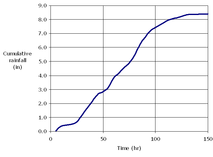
Figure 4-13. Example mass rainfall curve from historical storm
Hyetograph Development Procedure
In the rational method, the intensity is considered to be uniform over the storm period. Hydrograph techniques, however, account for variability of the intensity throughout a storm. Therefore, when using hydrograph techniques, the designer must determine a rainfall hyetograph: a temporal distribution of the watershed rainfall, as shown in Figure 4-14.
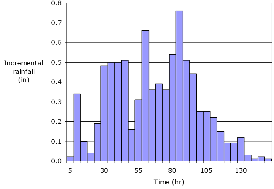
Figure 4-14. Rainfall hyetograph
Methods acceptable for developing a rainfall hyetograph for a design storm include the
method, the balanced storm method, and the Texas storm method.
NRCS Hyetograph Development Procedure
The NRCS design storm hyetographs were derived by averaging storm patterns for regions of the U.S. The storms thus represent a pattern distribution of rainfall over a 24-hour period to which a design rainfall depth can be applied. The distribution itself is arranged in a critical pattern with the maximum precipitation period occurring just before the midpoint of the storm.
The Natural Resources Conservation Service (NRCS) National Engineering Handbook (NEH), Part 630, Chapter 4 includes a detailed discussion on updating the temporal distribution of rainfall based on the new NOAA Atlas 14 rainfall data from the older NRCS Type II-III distributions commonly used in Texas, through 2019. TxDOT is evaluating whether to develop certain statewide temporal distribution zones similar to what Type II-III provided and further guidance may be forthcoming. Meanwhile, continued use of Type II and III temporal distribution of rainfall for Texas is no longer recommended, and the balanced storm method (also known as Frequency storm in HEC-HMS) is now preferred based on NRCS recommendations (NEH, Part 630.04).
Balanced Storm Hyetograph Development Procedure
The temporal distribution, with the peak of the storm located at the center of the hyetograph, is also called balanced storm. It uses DDF values that are based on a statistical analysis of historical data.
HEC-HMS software can derive hyetographs with the balanced method when the center of the storm is specified to be at 50% of the total storm duration. HEC-HMS also provides the ability to shift the peak from 50% of the total storm duration to 25%, 33%, 67%, or 75% as well, while maintaining the "nested" effect of the balanced storm.
The procedure for deriving a hyetograph with this method is as follows:
- For the selected , tabulate rainfall amounts for a storm of a given return period for all durations up to a specified limit (for 24-hour, 15-minute, 30-minute, 1-hour, 2-hour, 3-hour, 6-hour, 12-hour, 24-hour, etc.). Use for the duration and AEP selected for design.
- Select an appropriate time interval. An appropriate time interval is related to the time of concentration of the watershed. To calculate the time interval, use:
 Equation 4-25.Where:
- Dt= time interval
- t= time of concentrationc
- For example, if the time of concentration is 1 hour, Δt = 1/5tc= 1/5 of 1 hour = 12 minutes, or 1/6 of 1 hour = 10 minutes. Choosing 1/5 or 1/6 will not make a significant difference in the distribution of the rainfall; use one fraction or the other to determine a convenient time interval.
- For successive times of interval Δt, find the cumulative rainfall depths from the DDF values. For depths at time intervals not included in the DDF tables, interpolate depths for intermediate durations using a log-log interpolation. (Durations from the table are usually given in hours, but in minutes on the plot.) For example, given a study area in the northern part of Bexar County, the log-log plot in Figure 4-15 shows the 10% depths for the 15-, 30-, 60-, 120-, 180-, 360-, 720-, and 1440-minute durations included in Asquith and Roussel 2004. The precipitation depth at 500 minutes is interpolated as 5.0 inches.
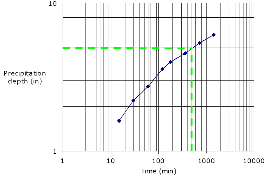 Figure 4-15. Log time versus log precipitation depth
 - Find the incremental depths by subtracting the cumulative depth at a particular time interval from the depth at the previous time interval.
- Rearrange the incremental depths so that the peak depth is at the center of the storm and the remaining incremental depths alternate (to left and right of peak) in descending order.
For example, in Figure 4-16, the largest incremental depth for a 24-hour storm (1,440 minutes) is placed at the 720-minute time interval and the remaining incremental depths are placed about the 720-minute interval in alternating decreasing order.
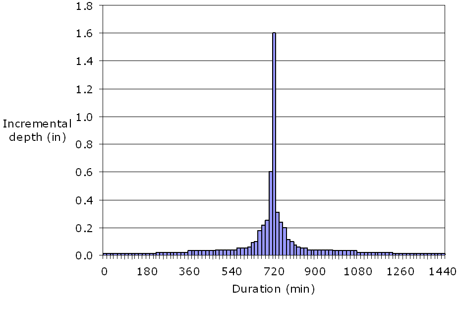
Figure 4-16. Balanced storm hyetograph
Texas Storm Hyetograph Development Procedure
Texas specific dimensionless hyetographs were developed by researchers at
,
,
, and
(Williams-Sether et al. 2004, Asquith et al. 2005). Two databases were used to estimate the hyetographs: 1) rainfall recorded for more than 1,600 storms over mostly small watersheds as part of historical USGS studies, and 2) hourly rainfall data collection network from the NWS over eastern New Mexico, Oklahoma, and Texas.
Three methods of developing dimensionless hyetographs are presented: 1) triangular dimensionless hyetograph; 2) L-gamma dimensionless hyetograph; and 3) empirical dimensionless hyetograph. Any of these hyetographs can be used for TxDOT design. Brief descriptions of the three methods are presented here. For further information and example problems on the Texas hyetographs, refer to Asquith et al. 2005.
Triangular Dimensionless Hyetograph
A triangular dimensionless hyetograph is presented in Figure 4-17. The vertical axis represents relative rainfall intensity. The rainfall intensity increases linearly until the time of peak intensity, then decreases linearly until the end of the storm. The triangular hyetograph, in terms of relative cumulative storm depth, is defined by Equations 4-26 and 4-27, with values for parameters a and b provided in Table 4-13.
Equation 4-26.
Equation 4-27.
Where:
- p= normalized cumulative rainfall depth, (ranging from 0 to 1) for F ranging from 0 to a1
- p2= normalized cumulative rainfall depth, (ranging from 0 to 1) for F ranging from a to 1
- F= elapsed time, relative to storm duration, ranging from 0 to 1
- a= relative storm duration prior to peak intensity, from Table 4-13
- b= relative storm duration prior to peak intensity, from Table 4-13
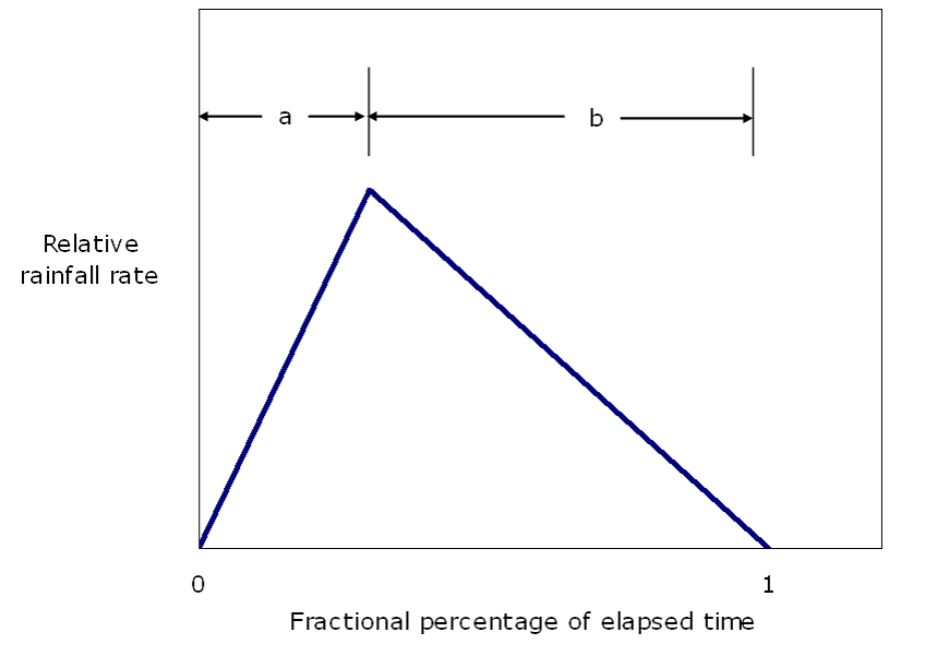
Figure 4-17. Triangular dimensionless Texas hyetograph
Triangular hyetograph model parameters | Storm duration | ||
|---|---|---|---|
5-12 hours | 13-24 hours | 25-72 hours | |
a | 0.02197 | 0.28936 | 0.38959 |
b | 0.97803 | 0.71064 | 0.61041 |
Based on the storm duration, the designer selects the appropriate parameters a and b for use in Equations 4-26 and 4-27. The ordinates of cumulative storm depth, normalized to total storm depth, are thus obtained. Values of rainfall intensity are obtained by computing total storm depth for durations of interest, and dividing by the duration.
Triangular Dimensionless Hyetograph Procedure
The following is an example computation using the triangular dimensionless hyetograph procedure for a 12-hour storm with cumulative depth of 8 inches:
- Express F in Equations 4-26 and 4-27 in terms of time t and total storm duration T: F = t / T.
- Express p in terms of cumulative rainfall depth d and total storm depth D: p = d / D.
- Substituting into Equations 4-26 and 4-27 gives:
- From Table 4-13, a = 0.02197 and b = 0.97803.

- Substituting 12 (hours) for T and 8 (inches) for D gives:

- Simplifying:

These resulting equations provide cumulative depth in inches as a function of elapsed time in hours, as shown in Table 4-14.
Time, t (hr.) | Precipitation Depth, d (in.) | Precipitation Intensity, I (in./hr.) |
|---|---|---|
0 | 0 | 0 |
0.13 | 0.04 | 0.33 |
0.26 | 0.17 | 0.99 |
0.50 | 0.49 | 1.32 |
0.75 | 0.81 | 1.29 |
1.00 | 1.13 | 1.26 |
2.00 | 2.32 | 1.19 |
3.00 | 3.40 | 1.08 |
4.00 | 4.36 | 0.97 |
5.00 | 5.22 | 0.85 |
6.00 | 5.96 | 0.74 |
7.00 | 6.58 | 0.62 |
8.00 | 7.09 | 0.51 |
9.00 | 7.49 | 0.40 |
10.00 | 7.77 | 0.28 |
11.00 | 7.94 | 0.17 |
12.00 | 8.00 | 0.06 |
L-gamma Dimensionless Hyetograph
Asquith (2003) and Asquith et al. (2005) computed sample L-moments of 1,659 dimensionless hyetographs for runoff-producing storms. Storms were divided by duration into 3 categories, 0 to 12 hours, 12 to 24 hours, and 24 to 72 hours. Dimensionless hyetographs based on the L-gamma distribution were developed and are defined by:
Equation 4-28.
Where:
- e= 2.718282
- p= normalized cumulative rainfall depth, ranging from 0 to 1
- F= elapsed time, relative to storm duration, ranging from 0 to 1
- b= distribution parameter from Table 4-15
- c= distribution parameter from Table 4-15
Parameters b and c of the L-gamma distribution for the corresponding storm durations are shown in Table 4-15. Until specific guidance is developed for selecting parameters for storms of exactly 12 hours and 24 hours, the designer should adopt distribution parameters for the duration range resulting in the more severe runoff condition.
Storm duration | L-gamma distribution parameters | |
|---|---|---|
b | c | |
0 – 12 hours | 1.262 | 1.227 |
12 – 24 hours | 0.783 | 0.4368 |
24 - 72 hours | 0.3388 | -0.8152 |
L-gamma Dimensionless Hyetograph Procedure
Use the following steps to develop an L-gamma dimensionless Texas hyetograph for storm duration of 24 hours and a storm depth of 15 inches:
- Enter the L-gamma distribution parameters for the selected storm duration into the following equation:
- Express F in terms of time t and total storm duration T: F = t / T. Express p in terms of cumulative rainfall depth d and total storm depth D: p = d / D. Substituting gives:
- Substitute 24 (hours) for T and 15 (inches) for D:
This equation defines the storm hyetograph. d is the cumulative depth in inches, and t is the elapsed time in hours.
Empirical Dimensionless Hyetograph
Empirical dimensionless hyetographs (Williams-Sether et al. 2004, Asquith et al. 2005) have been developed for application to small drainage areas (less than approximately 160 square miles) in urban and rural areas in Texas. The cumulative hyetographs are dimensionless in both duration and depth, and are applicable for storm durations ranging from 0 to 72 hours. The hyetograph shapes are not given by a mathematical expression but are provided graphically for 1
st
, 2nd
, 3rd
, and 4th
quartile storms as well as for a combined (1st
through 4th
quartile) storm.To use the hyetographs, the designer determines the appropriate storm depth and duration for the annual exceedance probability (AEP) of interest. The quartile defines in which temporal quarter of the storm the majority of the precipitation occurs – the graphs for individual quartiles as well as corresponding tabulations are available in
.
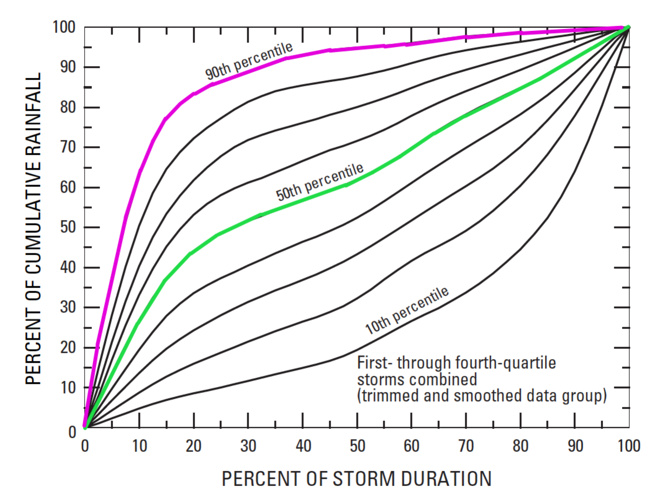
Figure 4-18. Dimensionless hyetographs for 0 to 72 hours storm duration (from Williams-Sether et al. 2004)
Storm duration (%) | 50 th Percentile Depth (%) | 90 th Percentile Depth (%) |
|---|---|---|
0.00 | 0.00 | 0.00 |
2.50 | 8.70 | 21.60 |
5.00 | 13.58 | 37.57 |
7.50 | 20.49 | 51.55 |
10.0 | 26.83 | 63.04 |
12.5 | 32.42 | 71.66 |
15.0 | 37.21 | 77.38 |
17.5 | 41.00 | 80.89 |
20.0 | 44.11 | 83.32 |
22.5 | 46.55 | 85.01 |
25.0 | 48.54 | 86.35 |
27.5 | 50.23 | 87.66 |
30.0 | 51.68 | 88.96 |
32.5 | 52.9 | 90.18 |
35.0 | 54.27 | 91.29 |
37.5 | 55.49 | 92.25 |
40.0 | 56.80 | 93.05 |
42.5 | 58.03 | 93.72 |
45.0 | 59.31 | 94.24 |
47.5 | 60.49 | 94.64 |
50.0 | 61.97 | 94.92 |
52.5 | 63.51 | 95.18 |
55.0 | 65.39 | 95.40 |
57.5 | 67.56 | 95.70 |
60.0 | 69.85 | 96.06 |
62.5 | 72.11 | 96.47 |
65.0 | 74.32 | 96.9 |
67.5 | 76.38 | 97.32 |
70.0 | 78.21 | 97.68 |
72.5 | 80.00 | 97.97 |
75.0 | 81.61 | 98.19 |
77.5 | 83.25 | 98.38 |
80.0 | 84.84 | 98.56 |
82.5 | 86.54 | 98.72 |
85.0 | 88.30 | 98.90 |
87.5 | 90.21 | 99.09 |
90.0 | 92.18 | 99.29 |
92.5 | 94.22 | 99.49 |
95.0 | 96.21 | 99.70 |
97.5 | 98.21 | 99.92 |
100.0 | 100.00 | 100.00 |
Figure 4-18 is a graphical representation of the combined storm with the 50th percentile (green) and 90th percentile (magenta) storm hyetograph highlighted, and Table 4-17 is the corresponding tabulation for a 50th percentile (median) storm and a 90th percentile storm. The recommended 50th percentile curve represents a median combined (1
st
through 4th
quartile) storm. The 90th percentile curve represents an upper support combined (1st
through 4th
quartile) storm where 90 percent of hyetographs would be anticipated to track either on or below the curve.Confidence limits for the empirical dimensionless hydrographs have been computed for each of the four quartile hyetographs and are reported in
. Because the hyetographs are dimensionless, all of the percentile hyetographs have the same dimensionless storm depth but represent variations in the temporal distribution of rainfall during the storm duration.
A spreadsheet tool,
(developed by
) is available to facilitate the use of the dimensionless hyetograph. It will assist the designer in producing elapsed time in minutes (or hours) and cumulative depth in inches (or millimeters) for the 50th or 90th percentile hyetograph. A
for use of the tool is included in
. The tool can also be used in conjunction with the
spread sheet.
Models for Estimating Losses
Losses refer to the volume of rain falling on a watershed that does not run off. With each model, precipitation loss is found for each computation time interval, and is subtracted from the precipitation depth for that interval. The remaining depth is referred to as precipitation excess. This depth is considered uniformly distributed over a watershed area, so it represents a volume of runoff.
Loss models available to the TxDOT designer include:
- Initial and constant-rate loss model.
- Texas initial and constant-rate loss model.
- curve number loss model.
- Green and Ampt loss model.
Initial and Constant-Rate Loss Model
Basic Concepts and EquationsFor the initial loss and constant–rate loss model, no runoff occurs in the watershed until an initial loss capacity has been satisfied, regardless of the rainfall rate. Once the initial loss has been satisfied, a constant potential loss rate occurs for the duration of the storm. This method is a simple approximation of a typical infiltration curve, where the initial loss decays over the storm duration to a final near-constant loss rate. In the example in Figure 4-19, the initial loss is satisfied in the first time increment, and the constant rate accounts for losses thereafter.
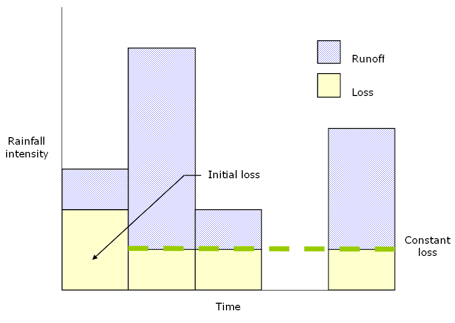
Figure 4-19. Initial and constant-loss rate model
The initial and constant loss-rate model is described mathematically as:
Equation 4-29.

Equation 4-30.

Equation 4-31.
Where:
- I(t)= rainfall intensity (in./hr.)
- f(t)= loss rate (in./hr.)
- P(t)= cumulative rainfall depth (in.) at time t
- I= initial loss (in.)a
- L= constant loss rate (in./hr.)
I
a
accounts for interception and depression storage, and the initial rate of infiltration at the beginning of the storm event. Interception refers to the capture of rainfall on the leaves and stems of vegetation before it reaches the ground surface. Depression storage is where the ponded rainfall fills small depressions and irregularities in the ground surface. Depression storage eventually infiltrates or evaporates during dry-weather periods. Until the accumulated precipitation on the pervious area exceeds the initial loss volume, no runoff occurs.Estimating Initial Loss and Constant Rate
The initial and constant-rate loss model includes one parameter (the constant rate) and one initial condition (the initial loss). Respectively, these represent physical properties of the watershed soils and land use and the antecedent condition.
If the watershed is in a saturated state, I
a
will approach 0. If the watershed is dry, then Ia
will increase to represent the maximum precipitation depth that can fall on the watershed with no runoff; this will depend on the watershed terrain, land use, soil types, and soil treatment.The constant loss rate can be viewed as the ultimate infiltration capacity of the soils. The
classified soils on the basis of this infiltration capacity as presented in Table 4-17; values in Column 4 represent reasonable estimates of the rates.
Texas Initial and Constant-Rate Loss Model
Recent research (TxDOT 0-4193-7) developed four computational approaches for estimating initial abstraction (I
A
) and constant loss (CL
) values for watersheds in Texas. The approaches are all based on the analysis of rainfall and runoff data of 92 gauged watersheds in Texas. One of those methods, presented here, allows the designer to compute IA
and CL
from regression equations:
Equation 4-32.

Equation 4-33.
Where:
- I= initial abstraction (in.)A
- C= constant loss rate (in./hr.)L
- L= main channel length (mi.)
- D= 0 for undeveloped watersheds, 1 for developed watersheds
- R= 0 for non-rocky watersheds, 1 for rocky watersheds
- CN= NRCS curve number
In the above equations, L is defined as “the length in stream-course miles of the longest defined channel shown in a 30-meter digital elevation model from the approximate watershed headwaters to the outlet” (TxDOT 0-4193-7).
NRCS Curve Number Loss Model
has developed a procedure to divide total depth of rainfall into soil retention, initial abstractions, and effective rainfall. This parameter is referred to as a curve number (CN). The CN is based on soil type, land use, and vegetative cover of the watershed. The maximum possible soil retention is estimated using a parameter that represents the impermeability of the land in a watershed. Theoretically, CN can range from 0 (100% rainfall infiltration) to 100 (impervious). In practice, based on values tabulated in NRCS 1986, the lowest CN the designer will likely encounter is 30, and the maximum CN is 98.
The CN may also be adjusted to account for wet or dry antecedent moisture conditions. Dry soil conditions are referred to as CN I, average conditions (those calculated using Estimating the CN) are referred to as CN II, and wet soils are referred to as CN III. Antecedent moisture conditions should be estimated considering a minimum of a five-day period. Antecedent soil moisture conditions also vary during a storm; heavy rain falling on a dry soil can change the soil moisture condition from dry to average to wet during the storm period.
Equation 4-34.
Equation 4-35.
Hydrologic Soil Groups
Soil properties influence the relationship between rainfall and runoff by affecting the rate of infiltration. NRCS divides soils into four hydrologic soil groups based on infiltration rates (Groups A-D). Urbanization has an effect on soil groups, as well. See Table 4-17 for more information.
Soil group | Description | Soil type | Range of loss rates | |
|---|---|---|---|---|
(in./hr.) | (mm/hr.) | |||
A | Low runoff potential due to high infiltration rates even when saturated | Deep sand, deep loess, aggregated silts | 0.30-0.45 | 7.6-11.4 |
B | Moderately low runoff potential due to moderate infiltration rates when saturated | Shallow loess, sandy loam | 0.15-0.30 | 3.8-7.6 |
C | Moderately high runoff potential due to slow infiltration rates Soils in which a layer near the surface impedes the downward movement of water or soils with moderately fine to fine texture | Clay loams, shallow sandy loam, soils low in organic content, and soils usually high in clay | 0.05-0.15 | 1.3-3.8 |
D | High runoff potential due to very slow infiltration rates | Soils that swell significantly when wet, heavy plastic clays, and certain saline soils | 0.00-0.05 | 1.3 |
Estimating the CN
Rainfall infiltration losses depend primarily on soil characteristics and land use (surface cover). The NRCS method uses a combination of soil conditions and land use to assign runoff CNs. Suggested runoff curve numbers are provided in Table 4-18, Table 4-19, Table 4-20, and Table 4-21. Note that CNs are whole numbers.
For a watershed that has variability in land cover and soil type, a composite CN is calculated and weighted by area.
Cover type and hydrologic condition | Average percent impervious area | A | B | C | D |
|---|---|---|---|---|---|
Open space (lawns, parks, golf courses, cemeteries, etc.): | |||||
Poor condition (grass cover < 50%) | 68 | 79 | 86 | 89 | |
Fair condition (grass cover 50% to 75%) | 49 | 69 | 79 | 84 | |
Good condition (grass cover > 75%) | 39 | 61 | 74 | 80 | |
Paved parking lots, roofs, driveways, etc. (excluding right-of-way) | 98 | 98 | 98 | 98 | |
Streets and roads: | |||||
Paved; curbs and storm drains (excluding right-of-way) | 98 | 98 | 98 | 98 | |
Paved; open ditches (including right-of-way) | 83 | 89 | 92 | 93 | |
Gravel (including right-of-way) | 76 | 85 | 89 | 91 | |
Dirt (including right-of-way) | 72 | 82 | 87 | 89 | |
Western desert urban areas: | |||||
Natural desert landscaping (pervious areas only) | 63 | 77 | 85 | 88 | |
Artificial desert landscaping (impervious weed barrier, desert shrub with 1- to 2-in. sand or gravel mulch and basin borders) | 96 | 96 | 96 | 96 | |
Urban districts: | |||||
Commercial and business | 85 | 89 | 92 | 94 | 95 |
Industrial | 72 | 81 | 88 | 91 | 93 |
Residential districts by average lot size: | |||||
1/8 acre or less (townhouses) | 65 | 77 | 85 | 90 | 92 |
1/4 acre | 38 | 61 | 75 | 83 | 87 |
1/3 acre | 30 | 57 | 72 | 81 | 86 |
1/2 acre | 25 | 54 | 70 | 80 | 85 |
1 acre | 20 | 51 | 68 | 79 | 84 |
2 acres | 12 | 46 | 65 | 77 | 82 |
Developing urban areas: Newly graded areas (pervious area only, no vegetation) | 77 | 86 | 91 | 94 | |
Notes: Values are for average runoff condition, and I a = 0.2S. The average percent impervious area shown was used to develop the composite CNs. Other assumptions are: impervious areas are directly connected to the drainage system, impervious areas have a CN of 98, and pervious areas are considered equivalent to open space in good hydrologic condition. | |||||
Cover type | Treatment | Hydrologic condition | A | B | C | D |
|---|---|---|---|---|---|---|
Fallow | Bare soil | - | 77 | 86 | 91 | 94 |
Crop residue cover (CR) | Poor Good | 76 74 | 85 83 | 90 88 | 93 90 | |
Row crops | Straight row (SR) | Poor Good | 72 67 | 81 78 | 88 85 | 91 89 |
SR + CR | Poor Good | 71 64 | 80 75 | 87 82 | 90 85 | |
Contoured (C) | Poor Good | 70 65 | 79 75 | 84 82 | 88 86 | |
C + CR | Poor Good | 69 64 | 78 74 | 83 81 | 87 85 | |
Contoured & terraced (C&T) | Poor Good | 66 62 | 74 71 | 80 78 | 82 81 | |
C&T + CR | Poor Good | 65 61 | 73 70 | 79 77 | 81 80 | |
Small grain | SR | Poor Good | 65 63 | 76 75 | 84 83 | 88 87 |
SR + CR | Poor Good | 64 60 | 75 72 | 83 80 | 86 84 | |
C | Poor Good | 63 61 | 74 73 | 82 81 | 85 84 | |
C + CR | Poor Good | 62 60 | 73 72 | 81 80 | 84 83 | |
C&T | Poor Good | 61 59 | 72 70 | 79 78 | 82 81 | |
C&T + CR | Poor Good | 60 58 | 71 69 | 78 77 | 81 80 | |
Close-seeded or broadcast legumes or rotation meadow | SR | Poor Good | 66 58 | 77 72 | 85 81 | 89 85 |
C | Poor Good | 64 55 | 75 69 | 83 78 | 85 83 | |
C&T | Poor Good | 63 51 | 73 67 | 80 76 | 83 80 | |
Notes: Values are for average runoff condition, and I a = 0.2S. Crop residue cover applies only if residue is on at least 5% of the surface throughout the year. Hydrologic condition is based on a combination of factors affecting infiltration and runoff: density and canopy of vegetative areas, amount of year-round cover, amount of grass or closed-seeded legumes in rotations, percent of residue cover on land surface (good > 20%), and degree of roughness. Poor = Factors impair infiltration and tend to increase runoff. Good = Factors encourage average and better infiltration and tend to decrease runoff. | ||||||
Cover type | Hydrologic condition | A | B | C | D |
|---|---|---|---|---|---|
Pasture, grassland, or range-continuous forage for grazing | Poor Fair Good | 68 49 39 | 79 69 61 | 86 79 74 | 89 84 80 |
Meadow – continuous grass, protected from grazing and generally mowed for hay | - | 30 | 58 | 71 | 78 |
Brush – brush-weed-grass mixture, with brush the major element | Poor Fair Good | 48 35 30 | 67 56 48 | 77 70 65 | 83 77 73 |
Woods – grass combination (orchard or tree farm) | Poor Fair Good | 57 43 32 | 73 65 58 | 82 76 72 | 86 82 79 |
Woods | Poor Fair Good | 45 36 30 | 66 60 55 | 77 73 70 | 83 79 77 |
Farmsteads – buildings, lanes, driveways, and surrounding lots | - | 59 | 74 | 82 | 86 |
Notes: Values are for average runoff condition, and I a = 0.2S. Pasture: Poor is < 50% ground cover or heavily grazed with no mulch, Fair is 50% to 75% ground cover and not heavily grazed, and Good is > 75% ground cover and lightly or only occasionally grazed. Meadow: Poor is < 50% ground cover, Fair is 50% to 75% ground cover, Good is > 75% ground cover. Woods/grass: CNs shown were computed for areas with 50 percent grass (pasture) cover. Other combinations of conditions may be computed from CNs for woods and pasture. Woods: Poor = forest litter, small trees, and brush destroyed by heavy grazing or regular burning. Fair = woods grazed but not burned and with some forest litter covering the soil. Good = woods protected from grazing and with litter and brush adequately covering soil. | |||||
Cover type | Hydrologic condition | A | B | C | D |
|---|---|---|---|---|---|
Herbaceous—mixture of grass, weeds, and low-growing brush, with brush the minor element | Poor Fair Good | 80 71 62 | 87 81 74 | 93 89 85 | |
Oak-aspen—mountain brush mixture of oak brush, aspen, mountain mahogany, bitter brush, maple, and other brush | Poor Fair Good | 66 48 30 | 74 57 41 | 79 63 48 | |
Pinyon-juniper—pinyon, juniper, or both; grass understory | Poor Fair Good | 75 58 41 | 85 73 61 | 89 80 71 | |
Sagebrush with grass understory | Poor Fair Good | 67 51 35 | 80 63 47 | 85 70 55 | |
Saltbush, greasewood, creosote-bush, blackbrush, bursage, palo verde, mesquite, and cactus | Poor Fair Good | 63 55 49 | 77 72 68 | 85 81 79 | 88 86 84 |
Notes: Values are for average runoff condition, and I a = 0.2S. Hydrologic Condition: Poor = < 30% ground cover (litter, grass, and brush overstory), Fair = 30% to 70% ground cover, Good = > 70% ground cover. Curve numbers for Group A have been developed only for desert shrub. | |||||
Soil Retention
The potential maximum retention (S) is calculated as:
Equation 4-36.
Where:
- z= 10 for English measurement units, or 254 for metric
- CN= runoff curve number
Equation 4-36 is valid if S is less than the rainfall excess, defined as precipitation (P) minus runoff (R) or S < (P-R). This equation was developed mainly for small watersheds from recorded storm data that included total rainfall amount in a calendar day but not its distribution with respect to time. Therefore, this method is appropriate for estimating direct runoff from 24-hour or 1-day storm rainfall.
Initial Abstraction
The initial abstraction consists of interception by vegetation, infiltration during early parts of the storm, and surface depression storage.
Generally, I
a
is estimated as:
Equation 4-37.
Effective Rainfall Runoff Volume
The effective rainfall (or the total rainfall minus the initial abstractions and retention) used for runoff hydrograph computations can be estimated using:
Equation 4-38.
Where:
- Pe= accumulated excess rainfall (in.)
- Ia= initial abstraction before ponding (in.)
- P = total depth of rainfall (in.)
- S = potential maximum depth of water retained in the watershed (in.)
Substituting Equation 4-37, Equation 4-38 becomes:
Equation 4-39.
P
e
and P have units of depth, Pe
and P reflect volumes and are often referred to as volumes because it is usually assumed that the same depths occurred over the entire watershed. Therefore Pe
is considered the volume of direct runoff per unit area, i.e., the rainfall that is neither retained on the surface nor infiltrated into the soil. Pe
also can be applied sequentially during a storm to compute incremental precipitation for selected time interval Δt.Climatic Adjustment of CN
NRCS curve numbers, estimated (predicted) using the procedure described in
Estimating the CN
, may be adjusted to account for the variation of climate within Texas. The adjustment is applied as follows:
Equation 4-40.
Where:
- CN= CN adjusted for climateobs
- CN= Estimated CN from NRCS procedures described inpredEstimating the CN
- CN= Deviation of CNdevobsfrom CNpred= climatic adjustment factor
In two studies (Hailey and McGill 1983, Thompson et al. 2003) CN
dev
was computed for gauged watersheds in Texas as CNobs
- CNpred
based on historical rainfall and runoff volumes. These studies show that CNdev
varies by location within the state.The following excerpt (Thompson et al. 2003) guides the designer in selection and application of the appropriate climatic adjustment to the predicted CN.
Given the differences between CN
obs
and CNpred
, it is possible to construct a general adjustment to CNpred
such that an approximation of CNobs
can be obtained. The large amount of variation in CNobs
does not lend to smooth contours or function fits. There is simply an insufficient amount of information for these types of approaches. However, a general adjustment can be implemented using regions with a general adjustment factor. Such an approach was taken and is presented in Figure 4-20.The bulk of rainfall and runoff data available for study were measured near the I-35 corridor. Therefore, estimates for this region are the most reliable. The greater the distance from the majority of the watershed that were part of this study, then the more uncertainty must be implied about the results. For the south high plains, that area south of the Balcones escarpment, and the coastal plain, there was insufficient data to make any general conclusions.
Application of the tool is straightforward. For areas where adjustment factors are defined (see Figure 4-20) the analyst should:
- Determine CNpredusing the normal NRCS procedure.
- Find the location of the watershed on the design aid (Figure 4-21). Determine an adjustment factor from the design aid and adjust the curve number.
- Examine Figure 4-21 and find the location of the watershed. Use the location of the watershed to determine nearby study watersheds. Then refer to Figure 4-20 and Table 4-22, Table 4-23, Table 4-24, Table 4-25, and Table 4-26 and determine CNpredand CNobsfor study watersheds near the site in question, if any are near the watershed in question.
- Compare the adjusted curve number with local values of CNobs.
The result should be a range of values that are reasonable for the particular site.
As a comparison, the adjusted curve number from Hailey and McGill (Figure 4-22) can be used.
A lower bound equivalent to the curve number for AMC I (dry antecedent conditions), or a curve number of 60, whichever is greater, should be considered.
Note that CN values are whole numbers. Rounding of values of CN
pred
in the tables may be required.Judgment is required for application of any hydrologic tool. The adjustments presented on Figure 4-20 are no exception. A lower limit of AMC I may be used to prevent an overadjustment downward. For areas that have few study watersheds, the Hailey and McGill approach should provide some guidance on the amount of reduction to CN
pred
is appropriate, if any.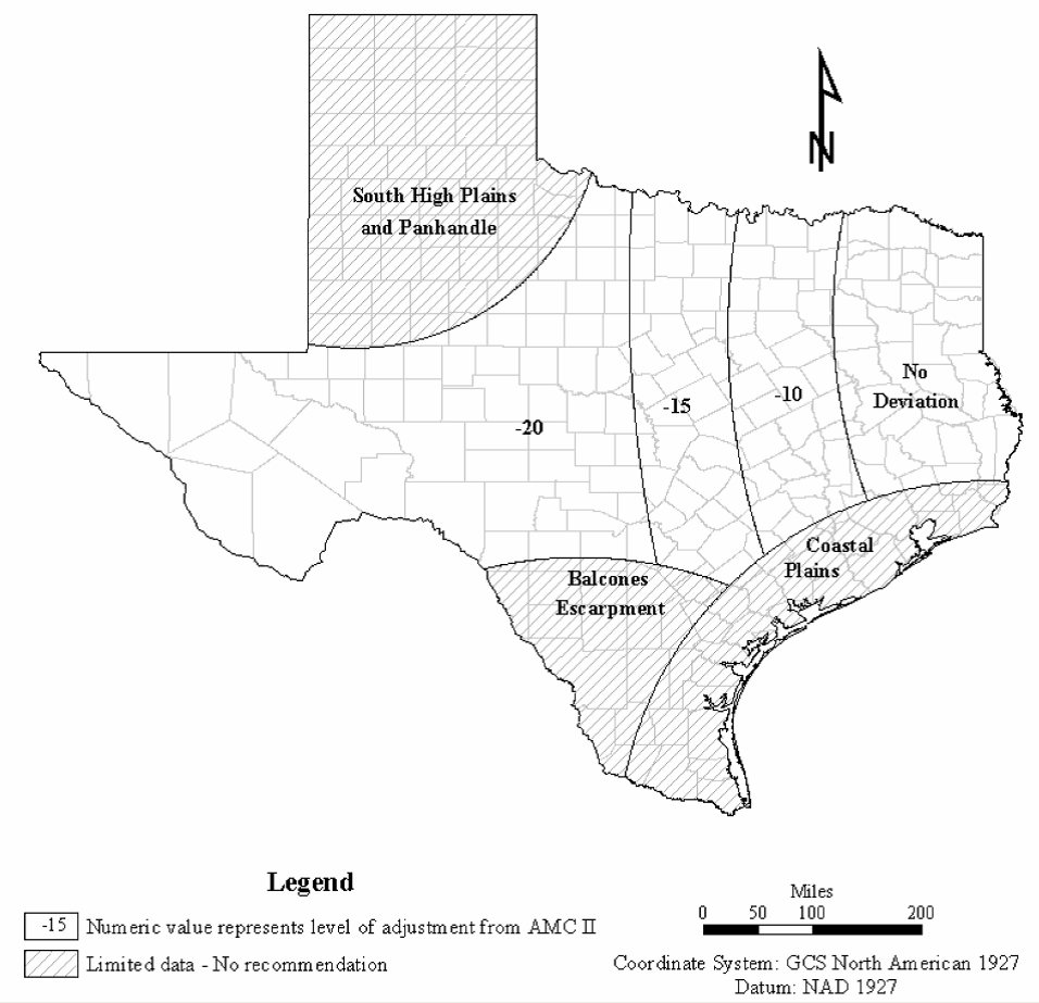
Figure 4-20. Climatic adjustment factor CN
dev
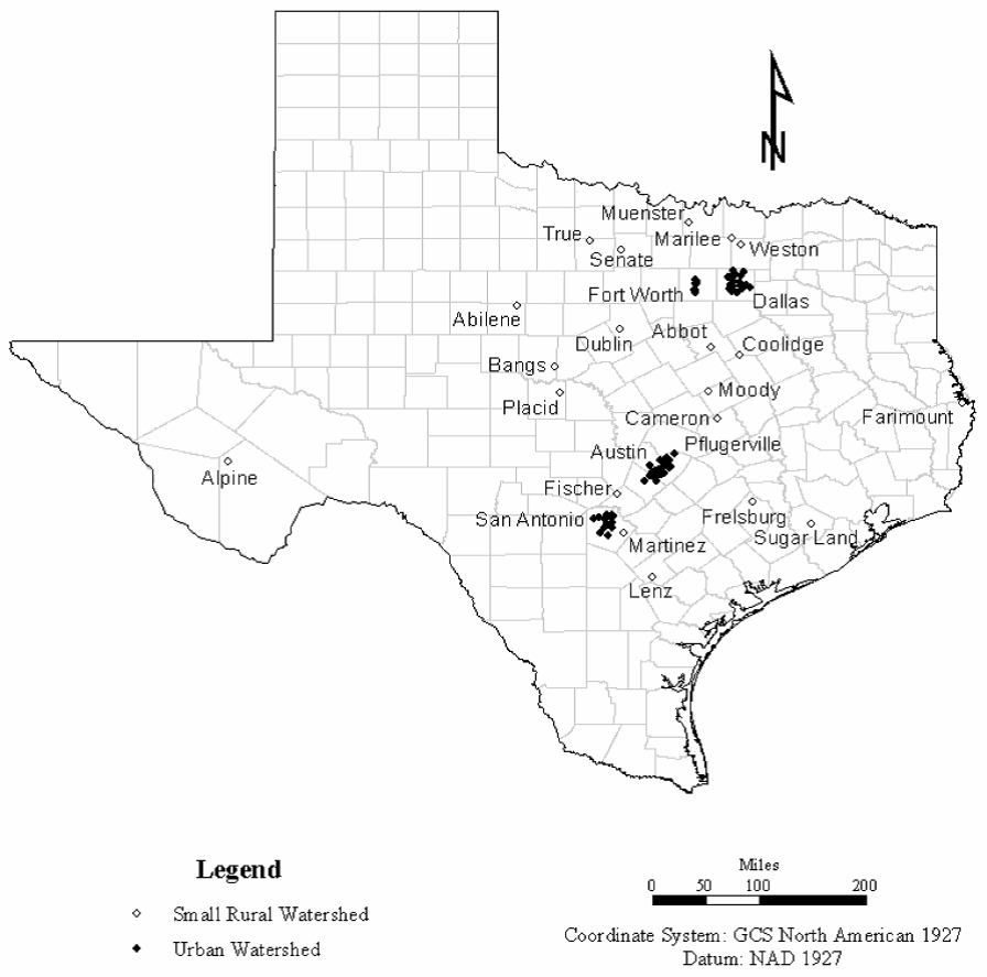
Figure 4-21. Location of CNdev watersheds
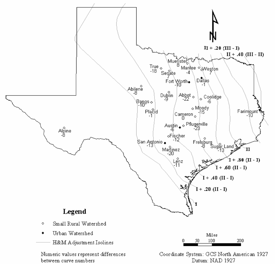
Climatic adjustment of CN - comparison of Hailey and McGill adjusted curve numbers, CNH&M, with CNobs. Negative differences indicate that CNH&M is larger than CNobs. Also shown are the lines of equal adjustment to curve number from Hailey and McGill’s (1983) Figure 4. (click in image to see full-size image)
USGS Gauge ID | Quad Sheet Name | CN obs | CN pred | CN dev |
|---|---|---|---|---|
8154700 | Austin West | 59 | 68.9 | -9.9 |
8155200 | Bee Cave | 65 | 70.7 | -5.7 |
8155300 | Oak Hill | 64 | 69.8 | -5.8 |
8155550 | Austin West | 50 | 87.3 | -37.3 |
8156650 | Austin East | 60 | 83.6 | -23.6 |
8156700 | Austin East | 78 | 86.6 | -8.6 |
8156750 | Austin East | 66 | 86.8 | -20.8 |
8156800 | Austin East | 66 | 87 | -21 |
8157000 | Austin East | 68 | 88.3 | -20.3 |
8157500 | Austin East | 67 | 89.1 | -22.1 |
8158050 | Austin East | 71 | 83.9 | -12.9 |
8158100 | Pflugerville West | 60 | 72.6 | -12.6 |
8158200 | Austin East | 62 | 75.6 | -13.6 |
8158400 | Austin East | 79 | 88.9 | -9.9 |
8158500 | Austin East | 71 | 85.6 | -14.6 |
8158600 | Austin East | 73 | 76.7 | -3.7 |
8158700 | Driftwood | 69 | 74.5 | -5.5 |
8158800 | Buda | 64 | 73.3 | -9.3 |
8158810 | Signal Hill | 64 | 69.8 | -5.8 |
8158820 | Oak Hill | 60 | 67.9 | -7.9 |
8158825 | Oak Hill | 49 | 67.2 | -18.2 |
8158840 | Signal Hill | 74 | 69.8 | 4.2 |
8158860 | Oak Hill | 60 | 68 | -8 |
8158880 | Oak Hill | 67 | 79.4 | -12.4 |
8158920 | Oak Hill | 71 | 77.5 | -6.5 |
8158930 | Oak Hill | 56 | 75.2 | -19.2 |
8158970 | Montopolis | 56 | 77.7 | -21.7 |
8159150 | Pflugerville East | 63 | 78.8 | -15.8 |
USGS Gauge ID | Quad Sheet Name | CN obs | CN pred | CN dev |
|---|---|---|---|---|
8055580 | Garland | 85 | 85.2 | -0.2 |
8055600 | Dallas | 82 | 86.1 | -4.1 |
8055700 | Dallas | 73 | 85.5 | -12.5 |
8056500 | Dallas | 85 | 85.8 | -0.8 |
8057020 | Dallas | 75 | 85.5 | -10.5 |
8057050 | Oak Cliff | 75 | 85.7 | -10.7 |
8057120 | Addison | 77 | 80.2 | -3.2 |
8057130 | Addison | 89 | 82.9 | 6.1 |
8057140 | Addison | 78 | 86.8 | -8.8 |
8057160 | Addison | 80 | 90.3 | -10.3 |
8057320 | White Rock Lake | 85 | 85.7 | -0.7 |
8057415 | Hutchins | 73 | 87.8 | -14.8 |
8057418 | Oak Cliff | 85 | 79.1 | 5.9 |
8057420 | Oak Cliff | 80 | 81 | -1 |
8057425 | Oak Cliff | 90 | 82.9 | 7.1 |
8057435 | Oak Cliff | 82 | 81.1 | 0.9 |
8057440 | Hutchins | 67 | 79.1 | -12.1 |
8057445 | Hutchins | 60 | 86.5 | -26.5 |
8061620 | Garland | 82 | 85 | -3 |
8061920 | Mesquite | 85 | 86 | -1 |
8061950 | Seagoville | 82 | 85.3 | -3.3 |
Gauge ID | Quad Sheet Name | CN obs | CN pred | CN dev |
|---|---|---|---|---|
8048520 | Fort Worth | 72 | 82.3 | -10.3 |
8048530 | Fort Worth | 69 | 86.7 | -17.7 |
8048540 | Covington | 73 | 88 | -15 |
8048550 | Haltom City | 74 | 91.2 | -17.2 |
8048600 | Haltom City | 65 | 84.3 | -19.3 |
8048820 | Haltom City | 67 | 83.4 | -16.4 |
8048850 | Haltom City | 72 | 83 | -11 |
USGS Gauge ID | Quad Sheet Name | CN obs | CN pred | CN dev |
|---|---|---|---|---|
8177600 | Castle Hills | 70 | 84.8 | -14.8 |
8178300 | San Antonio West | 72 | 85.7 | -13.7 |
8178555 | Southton | 75 | 84.2 | -9.2 |
8178600 | Camp Bullis | 60 | 79.7 | -19.7 |
8178640 | Longhorn | 56 | 78.4 | -22.4 |
8178645 | Longhorn | 59 | 78.2 | -19.2 |
8178690 | Longhorn | 78 | 84.4 | -6.4 |
8178736 | San Antonio East | 74 | 92.3 | -18.3 |
8181000 | Helotes | 50 | 79.2 | -29.2 |
8181400 | Helotes | 56 | 79.8 | -23.8 |
8181450 | San Antonio West | 60 | 87.3 | -27.3 |
USGS Gauge ID | Quadrangle Sheet Name | CN obs | CN pred | CN dev |
|---|---|---|---|---|
8025307 | Fairmount | 53 | 55.4 | -2.4 |
8083420 | Abilene East | 65 | 84.7 | -19.7 |
8088100 | True | 60 | 85.9 | -25.9 |
8093400 | Abbott | 61 | 88.1 | -27.1 |
8116400 | Sugarland | 70 | 82.9 | -12.9 |
8159150 | Pflugerville East | 55 | 83.7 | -28.7 |
8160800 | Freisburg | 56 | 67.8 | -11.8 |
8167600 | Fischer | 51 | 74.3 | -23.3 |
8436520 | Alpine South | 64 | 86.4 | -22.4 |
8435660 | Alpine South | 48 | 86.7 | -38.7 |
8098300 | Rosebud | 88 | 80.5 | 7.5 |
8108200 | Yarrelton | 77 | 79.9 | -2.9 |
8096800 | Bruceville | 62 | 80 | -18 |
8094000 | Bunyan | 60 | 78.4 | -18.4 |
8136900 | Bangs West | 51 | 75.8 | -24.8 |
8137000 | Bangs West | 52 | 74.5 | -22.5 |
8137500 | Trickham | 53 | 76.5 | -23.5 |
8139000 | Placid | 53 | 74.6 | -21.6 |
8140000 | Mercury | 63 | 74.4 | -11.4 |
8182400 | Martinez | 52 | 80 | -28 |
8187000 | Lenz | 53 | 83.8 | -30.8 |
8187900 | Kenedy | 63 | 73.3 | -10.3 |
8050200 | Freemound | 80 | 79.6 | 0.4 |
8057500 | Weston | 80 | 78.2 | 1.8 |
8058000 | Weston | 86 | 80.1 | 5.9 |
8052630 | Marilee | 80 | 85.4 | -5.4 |
8052700 | Aubrey | 74 | 84.1 | -10.1 |
8042650 | Senate | 59 | 63.4 | -4.4 |
8042700 | Lynn Creek | 50 | 62.5 | -12.5 |
8042700 | Senate | 56 | 62 | -6 |
8042700 | Senate | 65 | 55.9 | 9.1 |
8063200 | Coolidge | 70 | 79.4 | -9.4 |
Green and Ampt Loss Model
Basic Concepts and Equations
The Green and Ampt loss model is based on a theoretical application of Darcy’s law. The model, first developed in 1911, has the form:
Equation 4-41.
Where:
- f= infiltration capacity (in./hr.)
- K= saturated hydraulic conductivity (permeability) (in./hr.)s
- S= soil water suction (in.)w
- θs= volumetric water content (water volume per unit soil volume) under saturated conditions
- θ= volumetric moisture content under initial conditionsi
- F= total accumulated infiltration (in.)
The parameters can be related to soil properties.
Assumptions underlying the Green and Ampt model are the following:
- As rain continues to fall and water infiltrates, the wetting front advances at the same rate throughout the groundwater system, which produces a well-defined wetting front.
- The volumetric water contents, θsand θi, remain constant above and below the wetting front as it advances.
- The soil-water suction immediately below the wetting front remains constant with both time and location as the wetting front advances.
To calculate the infiltration rate at a given time, the cumulative infiltration is calculated using Equation 4-42 and differences computed in successive cumulative values:
Equation 4-42.
Where:
- t= time (hr.)
Equation 4-42 cannot be solved explicitly. Instead, solution by numerical methods is required. Once F is solved for, the infiltration rate, f, can be solved using Equation 4-41. These computations are typically performed by hydrologic computer programs equipped with Green-Ampt computational routines. With these programs, the designer is required to specify θ
s
, Sw
, and Ks
.Estimating Green-Ampt Parameters
To apply the Green and Ampt loss model, the designer must estimate the volumetric moisture content, θ
s
, the wetting front suction head, Sw
, and the saturated hydraulic conductivity, Ks
. Rawls et al. (1993) provide Green-Ampt parameters for several USDA soil textures as shown in Table 4-27. A range is given for volumetric moisture content in parentheses with typical values for each also listed.Soil texture class | Volumetric moisture content under saturated conditions θ s | Volumetric moisture content under initial conditions θ i | Wetting front suction head S w | Saturated hydraulic conductivity K s |
|---|---|---|---|---|
Sand | 0.437 (0.374-0.500) | 0.417 (0.354-0.480) | 1.95 | 9.28 |
Loamy sand | 0.437 (0.363-0.506) | 0.401 (0.329-0.473) | 2.41 | 2.35 |
Sandy loam | 0.453 (0.351-0.555) | 0.412 (0.283-0.541) | 4.33 | 0.86 |
Loam | 0.463 (0.375-0.551) | 0.434 (0.334-0.534) | 3.50 | 0.52 |
Silt loam | 0.501 (0.420-0.582) | 0.486 (0.394-0.578) | 6.57 | 0.27 |
Sandy clay loam | 0.398 (0.332-0.464) | 0.330 (0.235-0.425) | 8.60 | 0.12 |
Clay loam | 0.464 (0.409-0.519) | 0.309 (0.279-0.501) | 8.22 | 0.08 |
Silty clay loam | 0.471 (0.418-0.524) | 0.432 (0.347-0.517) | 10.75 | 0.08 |
Sandy clay | 0.430 (0.370-0.490) | 0.321 (0.207-0.435) | 9.41 | 0.05 |
Silty clay | 0.479 (0.425-0.533) | 0.423 (0.334-0.512) | 11.50 | 0.04 |
Clay | 0.475 (0.427-0.523) | 0.385 (0.269-0.501) | 12.45 | 0.02 |
Capabilities and Limitations of Loss Models
Selecting a loss model and estimating the model parameters are critical steps in estimating runoff. Some pros and cons of the different alternatives are shown in Table 4-28. These are guidelines and should be used as such. The designer should be familiar with the models and the watershed where applied to determine which loss model is most appropriate.
Model | Pros | Cons |
|---|---|---|
Initial and constant-loss rate | Has been successfully applied in many studies throughout the US. Easy to set up and use. Model only requires a few parameters to explain the variation of runoff parameters. | Difficult to apply to ungauged areas due to lack of direct physical relationship of parameters and watershed properties. Model may be too simple to predict losses within event, even if it does predict total losses well. |
Texas initial and constant-loss rate | Developed specifically from Texas watershed data for application to sites in Texas. Method is product of recent and extensive research. Simple to apply. | Method is dependent on NRCS CN. Relatively new method, and not yet widely used. |
NRCS CN | Simple, predictable, and stable. Relies on only one parameter, which varies as a function of soil group, land use, surface condition, and antecedent moisture condition. Widely accepted and applied throughout the U.S. | Predicted values not in accordance with classical unsaturated flow theory. Infiltration rate will approach zero during a storm of long duration, rather than constant rate as expected. Developed with data from small agricultural watersheds in midwestern US, so applicability elsewhere is uncertain. Default initial abstraction (0.2S) does not depend upon storm characteristics or timing. Thus, if used with design storm, abstraction will be same with 0.5 AEP storm and 0.01 AEP storm. Rainfall intensity not considered. |
Green and Ampt | Parameters can be estimated for ungauged watersheds from information about soils. | Not widely used, less experience in professional community. |
Rainfall to Runoff Transform
After the design storm hyetograph is defined, and losses are computed and subtracted from rainfall to compute runoff volume, the time distribution and magnitude of runoff is computed with a rainfall to runoff transform.
Two options are described herein for these direct runoff hydrograph computations:
- Unit hydrograph (UH) model. This is an empirical model that relies on scaling a pattern of watershed runoff.
- Kinematic wave model. This is a conceptual model that computes the overland flow hydrograph method with channel routing methods to convert rainfall to runoff and route it to the point of interest.
Unit Hydrograph Method
A unit hydrograph for a watershed is defined as the discharge hydrograph that results from one unit depth of excess rainfall distributed uniformly, spatially and temporally, over a watershed for a duration of one unit of time. The unit depth of excess precipitation is one inch for English units. The unit of time becomes the time step of the analysis, and is selected as short enough to capture the detail of the storm temporal distribution and rising limb of the unit hydrograph.
The unit hydrograph assumes that the rainfall over a given area does not vary in intensity. If rainfall does vary, the watershed must be divided into smaller subbasins and varying rainfall applied with multiple unit hydrographs. The runoff can then be routed from subbasin to subbasin.
For each time step of the analysis, the unit hydrograph ordinates are multiplied by the excess rainfall depth. The resulting time-coincident ordinates from each resulting hydrograph are summed to produce the total runoff hydrograph for the watershed. This process is shown graphically in Figure 4-23. Hydrographs a, b, c, and d are 1-hour unit hydrographs multiplied by the depth of excess rainfall in the individual 1-hour time steps. The total runoff hydrograph resulting from 4 hours of rainfall is the sum of hydrographs a, b, c, and d.
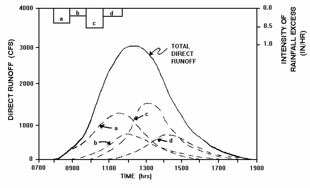
Figure 4-23. Unit hydrograph superposition (USACE 1994)
Mathematically, the computation of the runoff hydrograph is given by:
Equation 4-43.
Where:
- n = number of time steps
- Q= the runoff hydrograph ordinate n (at time nΔt)n
- P= effective rainfall ordinate m (in time interval mΔt)m
- △= computation time intervalt
- Q= unit hydrograph ordinate (n-m+1) (at time (n-m+1)Δt)u (n-m+1)
- m= number of periods of effective rainfall (of duration Δt)
- M = total number of discrete rainfall pulses
Equation 4-43 simplified becomes Q
1
= P1
U1
, Q2
= P1
U2
+P2
U1
, Q3
= P1
U3
+P2
U2
+P3
U1
, etc.Several different unit hydrograph methods are available to the designer. Each defines a temporal flow distribution. The time to peak flow and general shape of the distribution are defined by parameters specific to each method. The choice of unit hydrograph method will depend on available options within the hydrologic software being used, and also the availability of information from which to estimate the unit hydrograph parameters.
Two unit hydrograph methods commonly used by TxDOT designers are Snyder’s unit hydrograph and the NRCS unit hydrograph. These methods are supported by many rainfall-runoff software programs, which require the designer only to specify the parameters of the method. These two methods are discussed in the following sections.
Snyder’s Unit Hydrograph
Snyder developed a parametric unit hydrograph in 1938, based on research in the Appalachian Highlands using basins 10 to 10,000 square miles. Snyder’s unit hydrograph is described with two parameters: C
t
, which is a storage or timing coefficient; and Cp
, which is a peaking coefficient. As Ct
increases, the peak of the unit hydrograph is delayed. As Cp
increases, the magnitude of the unit hydrograph peak increases. Both Ct
and Cp
must be estimated for the watershed of interest. Values for Cp
range from 0.4 to 0.8 and generally indicate retention or storage capacity of the watershed.The peak discharge of the unit hydrograph is given by:
Equation 4-44.
Where:
- Q= peak discharge (cfs/in.)p
- A= drainage area (mi2)
- C= second coefficient of the Snyder method accounting for flood wave and storage conditionsp
- t= time lag (hr.) from the centroid of rainfall excess to peak of hydrographL
t
is given by:L
Equation 4-45.
Where:
- C= storage coefficient, usually ranging from 1.8 to 2.2t
- L= length of main channel (mi)
- L= length along the main channel from watershed outlet to the watershed centroid (mi)ca
The duration of excess rainfall (t
d
) can be computed using:
Equation 4-46.
Equation 4-46 implies that the relationship between lag time and the duration of excess rainfall is constant. To adjust values of lag time for other values of rainfall excess duration, the following equation should be used:
Equation 4-47.
Where:
- t= adjusted time lag (hr.)La
- t= alternative unit hydrograph duration (hr.)da
The time base of the unit hydrograph is a function of the lag time:
Equation 4-48.
Where:
- t= time base (days)b
The time to peak of the unit hydrograph is calculated by:
Equation 4-49.
Empirical relations of Snyder’s unit hydrograph were later found to aid the designer in constructing the unit hydrograph (McCuen 1989). The USACE relations, shown in Figure 4-24, are used to construct the Snyder unit hydrograph using the time to peak (t
p
), the peak discharge (Qp
), the time base (tb
), and 2 time parameters, W50
and W75
. W50
and W75
are the widths of the unit hydrograph at discharges of 50 percent and 75 percent of the peak discharge. The widths are distributed 1/3 before the peak discharge and 2/3 after.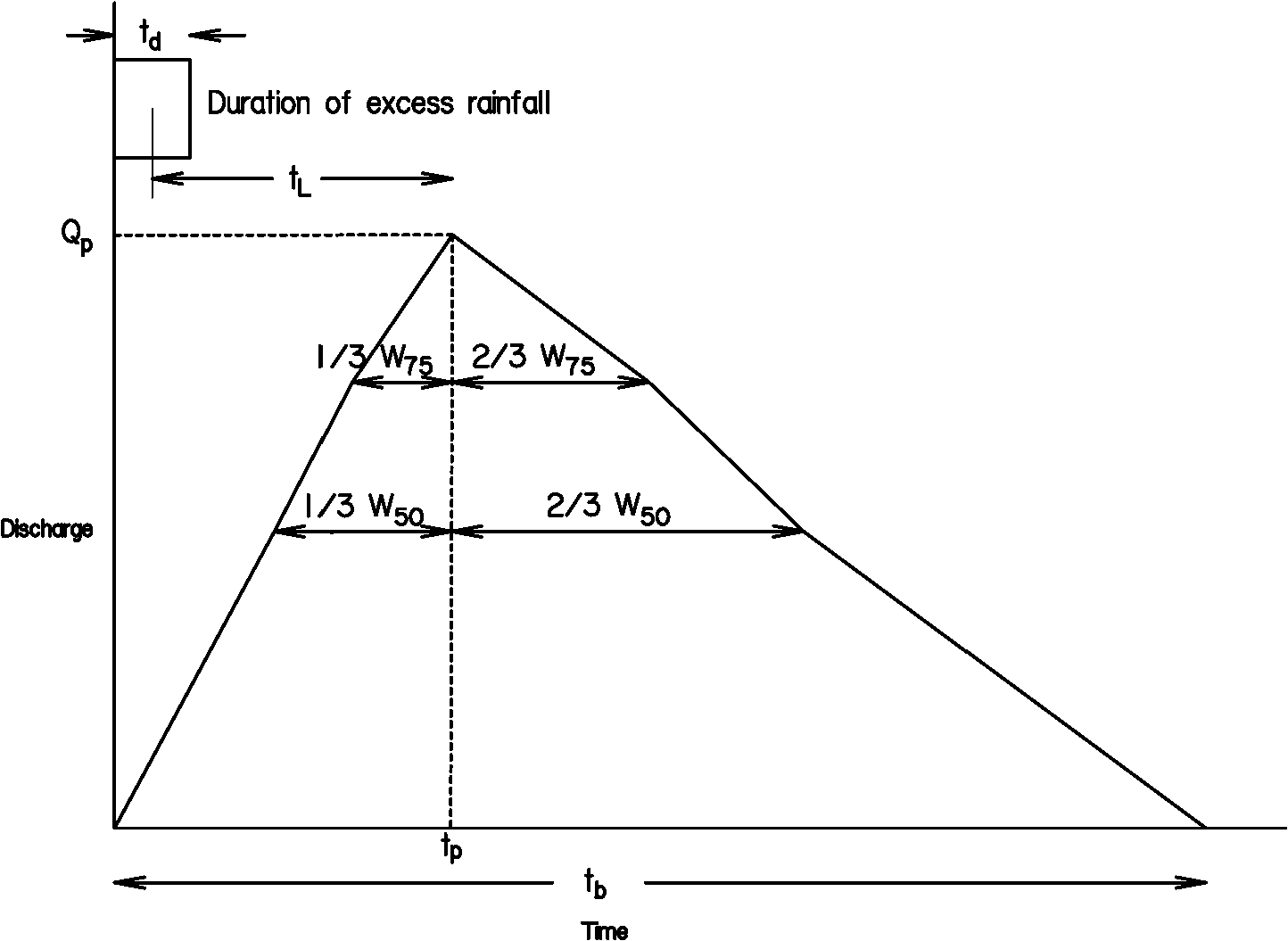
Figure 4-24. Snyder’s unit hydrograph
Values for W
50
and W75
are computed using these equations (McCuen 1989):
Equation 4-50.
Equation 4-51.
Where:
q
= peak discharge per square mile (i.e., Qa
p
/A, ft3
/sec/mi2
)NRCS Dimensionless Unit Hydrograph
The
unit hydrograph model is based upon an analysis and averaging of a large number of natural unit hydrographs from a broad cross section of geographic locations and hydrologic regions. For convenience, the hydrograph is dimensionless, with discharge ordinates (Q
u
) divided by the peak discharge (Qp
) and the time values (t) divided by the time to peak (tp
).The time-base of the dimensionless unit hydrograph is approximately five times the time to peak, and approximately 3/8 of the total volume occurs before the time to peak. The inflection point on the recession limb occurs at 1.67 times the time to peak, and the hydrograph has a curvilinear shape. The curvilinear hydrograph can be approximated by a triangular hydrograph with similar characteristics.
The curvilinear dimensionless NRCS unit hydrograph is shown in Figure 4-25.
Figure 4-25. NRCS dimensionless unit hydrograph
The ordinates of the dimensionless unit hydrograph are provided in Table 4-29.
t/t p | Q/Q p |
|---|---|
0.0 | 0.00 |
0.1 | 0.03 |
0.2 | 0.10 |
0.3 | 0.19 |
0.4 | 0.31 |
0.5 | 0.47 |
0.6 | 0.66 |
0.7 | 0.82 |
0.8 | 0.93 |
0.9 | 0.99 |
1.0 | 1.00 |
1.1 | 0.99 |
1.2 | 0.93 |
1.3 | 0.86 |
1.4 | 0.78 |
1.5 | 0.68 |
1.6 | 0.56 |
1.7 | 0.46 |
1.8 | 0.39 |
1.9 | 0.33 |
2.0 | 0.28 |
2.2 | 0.207 |
2.4 | 0.147 |
2.6 | 0.107 |
2.8 | 0.077 |
3.0 | 0.055 |
3.2 | 0.04 |
3.4 | 0.029 |
3.6 | 0.021 |
3.8 | 0.015 |
4.0 | 0.011 |
4.5 | 0.005 |
5.0 | 0.00 |
Notes: Variables are defined as follows: t = time (min.); t p = time to peak of unit hydrograph (min.);Q = discharge (cfs); and Q p = peak discharge of unit hydrograph (cfs). | |
The following procedure assumes the area or subarea is reasonably homogeneous. That is, the watershed is subdivided into homogeneous areas. The procedure results in a hydrograph only from the direct uncontrolled area. If the watershed has been subdivided, it might be necessary to perform hydrograph channel routing, storage routing, and hydrograph superposition to determine the hydrograph at the outlet of the watershed.
Application of the
dimensionless unit hydrograph to a watershed produces a site-specific unit hydrograph model with which storm runoff can be computed. To do this, the basin lag time must be estimated. The time to peak of the unit hydrograph is related to the lag time by:
Equation 4-52.
Where:
- t= time to peak of unit hydrograph (min.)p
- t= basin lag time (min.)L
- Dt= the time interval of the unit hydrograph (min.)
This time interval must be the same as the Δt chosen for the design storm.
The time interval may be calculated by:
Equation 4-53.
And the lag time is calculated by:
Equation 4-54.
The peak discharge of the unit hydrograph is calculated by:
Equation 4-55.
Where:
- Q= peak discharge (cfs)p
- C= conversion factor (645.33)f
- K= 0.75 (constant based on geometric shape of dimensionless unit hydrograph)
- A= drainage area (mi2); and
- t= time to peak (hr.)p
Equation 4-55 can be simplified to:
Equation 4-56.
The constant 484, or peak rate
factor (PRF)
, defines a unit hydrograph with 3/8 of its area under the rising limb. As the watershed slope becomes very steep (mountainous), the constant in Equation 4-56 can approach a value of approximately 600. For flat, swampy areas, the constant may decrease to a value 100 or lower (210-VI-NEH, March 2007)
. For applications in Texas, the use of the constant 484 is recommended as a starting point, but adjustments to a different value may be warranted. Limited sources are available for guidance on PRF adjustments. One source, while developed for the southeast US, provides practical guidance based on watershed size and slope (Sheridan, 2002). Any adjustments to the PRF must be well documented in the drainage report and model notes.
After t
p
and Qp
are estimated using Equations 4-52 and 4-56, the site specific unit hydrograph may be developed by scaling the dimensionless unit hydrograph.For each time step of the analysis, the site specific unit hydrograph ordinates are multiplied by the excess rainfall depth. The resulting hydrograph are summed to produce the total runoff hydrograph for the watershed. This process is shown graphically in Figure 4-23. While the computations can be completed using a spreadsheet model, a manual convolution can be somewhat time-consuming. These computations are typically performed by hydrologic computer programs.
For example, assume an area of 240 acres (0.375 sq. mi.) with T= 9 min, t
c
of 1.12 hours and CN of 80. For 1 inch of excess rainfall, △t
p
= 45 min, and Qp
= 243 cfs, using Equations 4-53, 4-52 and 4-56 respectively.Column 1 of Table 4-30 shows the time interval of 9 minutes. Column 2 is calculated by dividing the time interval by t
p
, in this case 45 minutes. Values in Column 3 are found by using the t/tp
value in Column 2 to find the associated Qu
/Qp
value from the dimensionless unit hydrograph shown in Figure 4-25, interpolating if necessary. Column 4 is calculated by multiplying Column 3 by Qp
, in this case 243 cfs.Table 4-30: Example Site-specific Unit Hydrograph
t (min.) | t/t p | Q u /Qp | Q u (cfs) |
|---|---|---|---|
0 | 0.00 | 0.000 | 0 |
9 | 0.20 | 0.100 | 24 |
18 | 0.40 | 0.310 | 75 |
27 | 0.60 | 0.660 | 160 |
36 | 0.80 | 0.930 | 226 |
45 | 1.00 | 1.000 | 243 |
54 | 1.20 | 0.930 | 226 |
63 | 1.40 | 0.780 | 190 |
72 | 1.60 | 0.560 | 136 |
81 | 1.80 | 0.390 | 95 |
90 | 2.00 | 0.280 | 68 |
99 | 2.20 | 0.207 | 50 |
108 | 2.40 | 0.147 | 36 |
117 | 2.60 | 0.107 | 26 |
126 | 2.80 | 0.077 | 19 |
135 | 3.00 | 0.055 | 13 |
144 | 3.20 | 0.040 | 10 |
153 | 3.40 | 0.023 | 6 |
162 | 3.60 | 0.021 | 5 |
171 | 3.80 | 0.015 | 4 |
180 | 4.00 | 0.011 | 3 |
189 | 4.20 | 0.009 | 2 |
198 | 4.40 | 0.006 | 2 |
207 | 4.60 | 0.004 | 1 |
216 | 4.80 | 0.002 | 0 |
225 | 5.00 | 0 | 0 |
The example site-specific unit hydrograph is shown in Figure 4-26.
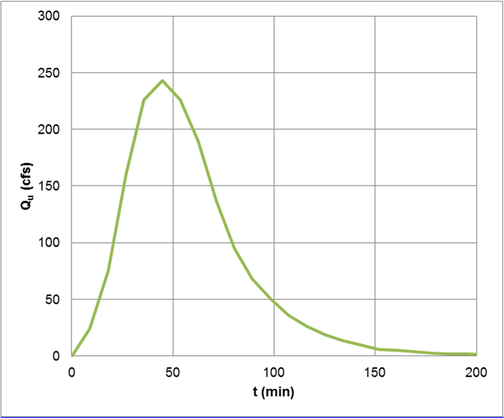
Figure 4-26. Example site-specific unit hydrograph
Remember that the site-specific hydrograph developed in Figure 4-26 was based on 1 inch of excess rainfall. For each time step of the analysis, the unit hydrograph ordinates are multiplied by the excess rainfall depth. Excess rainfall is obtained from a rainfall hyetograph such as a distribution developed from locally observed rainfall or the NRCS 24-hour, Type II or Type III rainfall distributions. The resulting hydrograph are summed to produce the total runoff hydrograph for the watershed. This process is shown graphically in Figure 4-24.
The capabilities and limitations of the NRCS unit hydrograph model include the following:
- This method does not account for variation in rainfall intensity or duration over the watershed.
- Baseflow is accounted for separately.
Kinematic Wave Overland Flow Model
A kinematic wave model is a conceptual model of watershed response that uses laws of conservation of mass and momentum to simulate overland and channelized flows. The model represents the watershed as a wide open channel, with inflow equal to the excess precipitation. Then it simulates unsteady channel flow over the surface to compute the watershed runoff hydrograph. The watershed is represented as a set of overland flow planes and collector channels.
In kinematic wave modeling, the watershed shown in Figure 4-27(a) is represented in Figure 4-27(b) as series of overland flow planes (gray areas) and a collector channel (dashed line). The collector channel conveys flow to the watershed outlet.
Figure 4-27. Kinematic wave model representation of a watershed (USACE 2000)
The equations used to define conservation of mass and momentum are the Saint Venant equations. The conservation of mass equation is:
Equation 4-57.
Where:
- A= cross sectional area of flow (ft2, m2)
- T= time (sec.)
- Q= flow rate (cfs, m3/sec.)
- x= distance along the flow path (ft, m)
- q= lateral discharge added to the flow path per unit length of the flow path (cfs/ft, mo3/sec./m)
The momentum equation energy gradient is approximated by:

Equation 4-58.
Where:
- a and b= coefficients related to the physical properties of the watershed.
Substituting Equation 4-56 into Equation 4-55 yields a single partial differential equation in Q:
Equation 4-59.
Where:
- q= lateral inflow (cfs/ft, mL3/s/m)
Equation 4-54 can be expressed in terms of Manning’s n, wetted perimeter, and bed slope by substituting the following expression for
α𝑄
into Equation 4-56:β
Equation 4-60.
Where:
- n= Manning’s roughness coefficient
- P= wetted perimeter (ft, m)
- S= flow plane slope (ft/ft, m/m)o
The solution to the resulting equation, its terms, and basic concepts are detailed in Chow (1959) and other texts.
Hydrograph Routing
In some cases, the watershed of interest will be divided into subbasins. This is necessary when ground conditions vary significantly between subbasin areas, or when the total watershed area is sufficiently large that variations in precipitation depth within the watershed must be modeled. A rainfall-runoff method (unit hydrograph or kinematic wave) will produce a flow hydrograph at the outlet of each subbasin. Before these hydrographs can be summed to represent flow at the watershed outlet, the effects of travel time and channel/floodplain storage between the subbasin outlets and watershed outlet must be accounted for. The process of starting with a hydrograph at a location and recomputing the hydrograph at a downstream location is called hydrograph routing.
Figure 4-28 shows an example of a hydrograph at upstream location A, and the routed hydrograph at downstream location B. The resulting delay in flood peak is the travel time of the flood hydrograph. The resulting decrease in magnitude of the flood peak is the attenuation of the flood hydrograph.
Figure 4-28. Hydrograph routing (USACE 1994)
There are two general methods for routing hydrographs: hydrologic and hydraulic. The methods are distinguished by which equations are solved to compute the routed hydrograph.
Hydrologic methods solve the equation of continuity (conservation of mass), and typically rely on a second relationship (such as relation of storage to outflow) to complete the solution. The equation of continuity can be written as:
Equation 4-61.
Where:
- I= average inflow to reach or storage area during Dt
- O= average outflow to reach or storage area during Dt
- S= storage in reach or storage area
- Dt= time step
Hydrologic methods are generally most appropriate for steep slope conditions with no significant backwater effects. Hydrologic routing methods include (USACE 1994):
- Modified Puls—for a single reservoir or channel modeled as series of level-pool reservoirs.
- Muskingum—channel modeled as a series of sloped-pool reservoirs.
- Muskingum-Cunge—enhanced version of Muskingum method incorporating channel geometry and roughness information.
Most hydrologic software applications capable of multi-basin analysis offer a selection of hydrologic routing methods.
Hydraulic routing methods solve the Saint Venant equations. These are the one-dimensional equations of continuity (Equation 4-60) and conservation of momentum (Equation 4-61) written for open-channel flow. The equations are valid for gradually varied unsteady flow.
The one-dimensional equation of continuity is:
Equation 4-62.
Where:
- A= cross-sectional flow area
- V= average velocity of water
- x= distance along channel
- B= water surface width
- y= depth of water
- t= time
- q= lateral inflow per unit length of channel
The one-dimensional equation of conservation of momentum is:
Equation 4-63.
Where:
- S= friction slopef
- S= channel bed slopeo
- g= acceleration due to gravity
Hydraulic routing methods are computationally more intensive than hydrologic methods and are distinguished by which terms in the momentum equation (Equation 4-61) are included (not neglected) in the solution algorithm. Hydraulic routing methods include (USACE 1994):
- Dynamic wave (all terms of St. Venant equations)
- Diffusion wave
- Kinematic wave
One-dimensional unsteady open-channel flow software applications implicitly route hydrographs from one location to another by solving for depth and velocity at all locations (cross sections) in a stream reach (or network of reaches) for every time step. The hydraulic routing method employed is defined by the solution algorithm of the software application. Some applications allow the user to select which hydraulic routing method is used, while other applications support only one method.
The most robust routing method (in terms of steep/mild stream slope and with/without backwater effects) is dynamic wave routing.
Selection of Routing Method
Selection of an appropriate routing method depends on several factors. The application of any method will be improved if observed data are available for calibration/verification of routing parameters. Generally, hydrologic methods are most suitable for steeper reaches having little or no backwater effects resulting from high stages downstream of the routing reach. Hydraulic methods are generally more appropriate for a wider range of channel slopes, including gradual slopes, and can accommodate backwater effects. The exception to this is the Muskingum-Cunge method, which does not perform well with steep-rising hydrographs in gradual slopes, or backwater conditions. Of all methods, only the dynamic wave routing method is appropriate for steep and gradual slopes, as well as with or without backwater conditions.
As a baseline approach, the designer may consider using the Muskingum-Cunge method in cases having steep slope (greater than 10 feet per mile) and no backwater effects. This method, which is described in Chow (1988) and Fread (1993), has the advantage that it will incorporate the shape of the cross section into computations. In some cases, cross section data may be obtained from existing hydraulic models of the reach. If channel geometry data are unavailable, then the Muskingum or modified Puls methods, which are described below, may be used. However, these two methods should be avoided for channel routing applications unless observed data are available for calibration/verification of routing parameters.
In cases having backwater that significantly affect the storage-outflow relationship of the routing reach, and thereby significantly affect the routed hydrograph, the dynamic wave, diffusion wave, and modified Puls methods are appropriate.
All methods, except for kinematic wave, are appropriate in cases having a channel slope between 2 to 10 feet per mile, no backwater effects, and satisfying the condition given by Equation 4-62 (USACE 1994):
Equation 4-64.
Where:
- T= hydrograph duration (s)
- S= average friction or slope (ft/ft)o
- u= mean velocity (ft/s)o
- d= average flow depth (ft)o
Only the dynamic wave, diffusion wave, and Muskingum-Cunge methods are appropriate in cases having a channel slope less than 2 feet per mile, no backwater effects, and satisfying the condition given by Equation 4-63 (USACE 1994):
Equation 4-65.
Where:
- g= 32.2 ft/s
In cases having a channel slope less than 2 feet per mile, no backwater effects, and not satisfying the condition given by Equation 4-63, then only the dynamic wave method is appropriate.
It may be tempting for the designer to select the dynamic wave routing method as a general approach for all conditions. However, the designer will find that the substantial amount of information (detailed and closely-spaced cross section geometry data) required to construct a one-dimensional unsteady flow model, and the significant time required to ensure that the model is running properly without numerical instabilities, will provide motivation to identify a suitable hydrologic routing method when appropriate. If hydrologic methods are not appropriate for the case under consideration, then an unsteady flow model may be required to properly route flows.
Reservoir Versus Channel Routing
Inflow hydrographs can be routed through reservoirs using a simple (single reservoir) hydrologic routing method, such as the modified Puls storage method. This is because the relationship between storage and discharge is unique (single-valued). In other words, the storage in the reservoir is fully described by the stage in the reservoir because the surface of the reservoir is the same shape and slope during the rising and falling limbs of the hydrograph.
Hydrologic routing methods may also be used for channel routing. A channel does not have a single-valued storage-outflow curve. Instead, the storage-outflow relation is looped, as shown in Figure 4-29. As a result, a hydrologic routing method employing a single reservoir representation cannot be used.
Figure 4-29. Looped storage outflow relation (USACE 1994)
The level-pool limitation of hydrologic routing methods is overcome by representing the channel as a series of reservoirs. These are termed subreaches, or steps, within the routing reach. Another enhancement to the level-pool approach, employed by the Muskingum method, is to represent the storage in each reservoir as a combination of prism storage (similar to level-pool reservoir) and wedge storage (additional sloped water on top of prism).
An estimate of the number of routing steps required for a hydrologic channel routing method is given by (USACE 1994):

Equation 4-66.
Where:
- n= number of routing steps
- K= floodwave travel time through the reach (min.)
- Dt= time step (min.)
K
in the above equation is given by:
Equation 4-67.
Where:
- L= length of routing reach (ft)
- V= flood wave velocity (ft/s)W
V
W
may be approximated as equal to the average channel velocity during the flood hydrograph. A better estimate of VW
is given by Seddon’s law applied to a cross section representative of the routing reach (USACE 1994):
Equation 4-68.
Where:
- B= top with of the channel water surface (ft)
- Q= channel discharge (cfs) as function of elevation y
 = slope of the discharge rating curve (ft2/s)
Two hydrologic routing methods and their application are discussed further in the following sections: the modified Puls method for reservoir routing, and the Muskingum method for channel routing.
Modified Puls Method Reservoir Routing
Basic Concepts and Equations
The basic storage routing equation states that mass is conserved and can be expressed as follows: Average inflow - average outflow = Rate of change in storage
In numerical form, this statement of flow continuity can be written as:
Equation 4-69.
Where:
- I= inflow at time step number tt
- I= inflow at time step number t + 1t+1
- O= outflow at time step number tt
- O= outflow at time step number t + 1t+1
- S= storage in the reservoir at time step number tt
- S= storage in the reservoir at time step number t + 1t+1
- Δt= the time increment
- Δt= the time increment *** REMOVE DUPLATE INFO IF DISPLAYS NICELY ***
- t= time step number
In Equation 4-64 there are two unknowns: O
t+1
and St+1
.
In order to solve Equation 4-64, either a second equation with Ot+1
and St+1
is required, or a relationship between Ot+1
and St+1
is needed.
The storage-indication approach is the latter and is presented here. First, it is convenient to rewrite the routing equation as:
Equation 4-70.
In this form, all terms known at time t are on the right hand side of the equation and unknowns are on the left. If a single-valued storage-outflow curve can be determined for the routing reach, then for any value of O
t+1
, the corresponding value of S
t+1
will be known. This reduces the number of unknown parameters in Equation 4-65 from two (Ot+1
and St+1
) to one (Ot+1
).Use of the storage routing method requires the designer to determine the relationship between storage and outflow. This is simply the volume of water held by the reservoir, storage facility, or pond as a function of the water surface elevation or depth. For a reservoir or storage facility, this information is often available from the reservoir sponsor or owner.
For a pond or lake or where the stage-storage relation is not available, a relationship between storage and outflow can be derived from considerations of physical properties of channel or pond and simple hydraulic models of outlet works or relationship of flow and water surface elevation. These physical properties include:
- Ratings of the primary and/or emergency spillway of a reservoir.
- Pump flow characteristics in a pump station.
- Hydraulic performance curve of a culvert or bridge on a highway.
- Hydraulic performance curve of a weir and orifice outlet of a detention pond.
With the stage-storage relation established, a storage indication curve corresponding to the left side of Equation 4-68 is developed. The relationship is described in the form of O versus (2S/ΔT) + O. An example of a storage indication curve is provided in Figure 4-30.
Figure 4-30. Sample storage-indication relation
The form of Equation 4-68 shown above is useful because the terms on the left side of the equation are known. With the relation between the outflow and storage determined (Figure 4-30), the ordinates on the outflow hydrograph can be determined directly.
Storage Routing Procedure
Use the following steps to route an inflow flood runoff hydrograph through a storage system such as a reservoir or detention pond:
- Acquire or develop a design flood runoff hydrograph for the project site watershed.
- Acquire or develop a stage-storage relation.
- Acquire or develop a stage-outflow relationship.
- Develop a storage-outflow relationship.
- Assume an initial value for Otas equal to It. At time step one (t = 1), assume an initial value for Otas equal to It. Usually, at time step one, inflow equals zero, so outflow will be zero and 2S1/ΔT - O1equals zero. Note that to start, t + 1 in the next step is 2.
- Compute 2St+1/ΔT + Ot+1using Equation 4-68.
- Interpolate to find the value of outflow. From the storage-outflow relation, interpolate to find the value of outflow (Ot+1) at (2St+1)/(ΔT)+Ot+1from step 6.
- Determine the value of (2St+1)/(ΔT)-Ot+1. Use the relation (2St+1)/(ΔT)-Ot+1= (2St+1)/(ΔT)+Ot+1- 2Ot+1.
- Assign the next time step to the value of t, e.g., for the first run through set t = 2.
- Repeat steps 6 through 9 until the outflow value (Ot+1) approaches zero.
- Plot the inflow and outflow hydrographs. The peak outflow value should always coincide with a point on the receding limb of the inflow hydrograph.
- Check conservation of mass to help verify success of the process. Use Equation 4-69 to compare the inflow volume to the sum of retained and outflow volumes:
 Equation 4-71.
Where:
- S= difference in starting and ending storage (ftr3or m3)
- SI= sum of inflow hydrograph ordinates (cfs or mt3/s)
- SO= sum of outflow hydrograph ordinates (cfs or mt3/s)
Muskingum Method Channel Routing
Routing of flood hydrographs by means of channel routing procedures is useful in instances where computed hydrographs are at points other than the points of interest. This is also true in those instances where the channel profile or plan is changed in such a way as to alter the natural velocity or channel storage characteristics. Routing estimates the effect of a channel reach on an inflow hydrograph. This section describes the Muskingum method equations, a lumped flow routing technique that approximates storage effects in the form of a prism and wedge component (Chow 1988).
The Muskingum method also solves the equation of continuity. With the Muskingum method, the storage in the channel is considered the sum of two components: prism storage and wedge storage (Figure 4-31).
Figure 4-31. Muskingum prism and wedge storage
The constants K and X are used to relate the prism component, KO, and wedge component, KX(I-O), to the inflow and outflow of the reach:
Equation 4-72.
Where:
- S= total storage (ft3or m3)
- K= a proportionality constant representing the time of travel of a flood wave to traverse the reach (s). Often, this is set to the average travel time through the reach.
- X= a weighting factor describing the backwater storage effects approximated as a wedge
- I= inflow (cfs or m3/s)
- O= outflow (cfs or m3/s)
The value of X depends on the amount of wedge storage; when X = 0, there is no backwater (reservoir type storage), and when X = 0.5, the storage is described as a full wedge. The weighting factor, X, ranges from 0 to 0.3 in natural streams. A value of 0.2 is typical.
Equation 4-68 represents the time rate of change of storage as the following:
Equation 4-73.
Where:
- DT= time interval usually ranging from 0.3K to K
- t= time step number
Combining Equation 4-70 with Equation 4-71 yields the Muskingum flow routing equation:
Equation 4-74.
Where:
Equation 4-75.
Equation 4-76.
Equation 4-77.
By definition, the sum of C, C
1
2
, and C3
is 1. If measured inflow and outflow hydrographs are available, K and X can be estimated using Equation 4-71. Calculate X by plotting the numerator on the vertical axis and the denominator on the horizontal axis, and adjusting X until the loop collapses into a single line. The slope of the line equals K:
Equation 4-78.
The designer may also estimate K and X using the Muskingum-Cunge method described in Chow 1988 or Fread 1993.