Rainfall to Runoff Transform
After the design storm hyetograph is defined, and losses are computed and subtracted from rainfall to compute runoff volume, the time distribution and magnitude of runoff is computed with a rainfall to runoff transform.
Two options are described herein for these direct runoff hydrograph computations:
- Unit hydrograph (UH) model. This is an empirical model that relies on scaling a pattern of watershed runoff.
- Kinematic wave model. This is a conceptual model that computes the overland flow hydrograph method with channel routing methods to convert rainfall to runoff and route it to the point of interest.
Unit Hydrograph Method
A unit hydrograph for a watershed is defined as the discharge hydrograph that results from one unit depth of excess rainfall distributed uniformly, spatially and temporally, over a watershed for a duration of one unit of time. The unit depth of excess precipitation is one inch for English units. The unit of time becomes the time step of the analysis, and is selected as short enough to capture the detail of the storm temporal distribution and rising limb of the unit hydrograph.
The unit hydrograph assumes that the rainfall over a given area does not vary in intensity. If rainfall does vary, the watershed must be divided into smaller subbasins and varying rainfall applied with multiple unit hydrographs. The runoff can then be routed from subbasin to subbasin.
For each time step of the analysis, the unit hydrograph ordinates are multiplied by the excess rainfall depth. The resulting time-coincident ordinates from each resulting hydrograph are summed to produce the total runoff hydrograph for the watershed. This process is shown graphically in Figure 4-23. Hydrographs a, b, c, and d are 1-hour unit hydrographs multiplied by the depth of excess rainfall in the individual 1-hour time steps. The total runoff hydrograph resulting from 4 hours of rainfall is the sum of hydrographs a, b, c, and d.
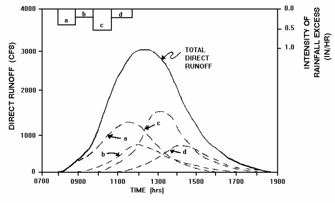
Figure 4-23. Unit hydrograph superposition (USACE 1994)
Mathematically, the computation of the runoff hydrograph is given by:
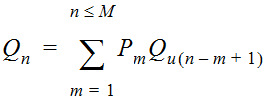
Equation 4-43.
Where:
- n = number of time steps
- Q= the runoff hydrograph ordinate n (at time nΔt)n
- P= effective rainfall ordinate m (in time interval mΔt)m
- △= computation time intervalt
- Q= unit hydrograph ordinate (n-m+1) (at time (n-m+1)Δt)u (n-m+1)
- m= number of periods of effective rainfall (of duration Δt)
- M = total number of discrete rainfall pulses
Equation 4-43 simplified becomes Q
1
= P1
U1
, Q2
= P1
U2
+P2
U1
, Q3
= P1
U3
+P2
U2
+P3
U1
, etc.Several different unit hydrograph methods are available to the designer. Each defines a temporal flow distribution. The time to peak flow and general shape of the distribution are defined by parameters specific to each method. The choice of unit hydrograph method will depend on available options within the hydrologic software being used, and also the availability of information from which to estimate the unit hydrograph parameters.
Two unit hydrograph methods commonly used by TxDOT designers are Snyder’s unit hydrograph and the NRCS unit hydrograph. These methods are supported by many rainfall-runoff software programs, which require the designer only to specify the parameters of the method. These two methods are discussed in the following sections.
Snyder’s Unit Hydrograph
Snyder developed a parametric unit hydrograph in 1938, based on research in the Appalachian Highlands using basins 10 to 10,000 square miles. Snyder’s unit hydrograph is described with two parameters: C
t
, which is a storage or timing coefficient; and Cp
, which is a peaking coefficient. As Ct
increases, the peak of the unit hydrograph is delayed. As Cp
increases, the magnitude of the unit hydrograph peak increases. Both Ct
and Cp
must be estimated for the watershed of interest. Values for Cp
range from 0.4 to 0.8 and generally indicate retention or storage capacity of the watershed.The peak discharge of the unit hydrograph is given by:
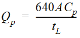
Equation 4-44.
Where:
- Q= peak discharge (cfs/in.)p
- A= drainage area (mi2)
- C= second coefficient of the Snyder method accounting for flood wave and storage conditionsp
- t= time lag (hr.) from the centroid of rainfall excess to peak of hydrographL
t
is given by:L
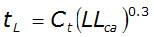
Equation 4-45.
Where:
- C= storage coefficient, usually ranging from 1.8 to 2.2t
- L= length of main channel (mi)
- L= length along the main channel from watershed outlet to the watershed centroid (mi)ca
The duration of excess rainfall (t
d
) can be computed using:
Equation 4-46.
Equation 4-46 implies that the relationship between lag time and the duration of excess rainfall is constant. To adjust values of lag time for other values of rainfall excess duration, the following equation should be used:
Equation 4-47.
Where:
- t= adjusted time lag (hr.)La
- t= alternative unit hydrograph duration (hr.)da
The time base of the unit hydrograph is a function of the lag time:
Equation 4-48.
Where:
- t= time base (days)b
The time to peak of the unit hydrograph is calculated by:
Equation 4-49.
Empirical relations of Snyder’s unit hydrograph were later found to aid the designer in constructing the unit hydrograph (McCuen 1989). The USACE relations, shown in Figure 4-24, are used to construct the Snyder unit hydrograph using the time to peak (t
p
), the peak discharge (Qp
), the time base (tb
), and 2 time parameters, W50
and W75
. W50
and W75
are the widths of the unit hydrograph at discharges of 50 percent and 75 percent of the peak discharge. The widths are distributed 1/3 before the peak discharge and 2/3 after.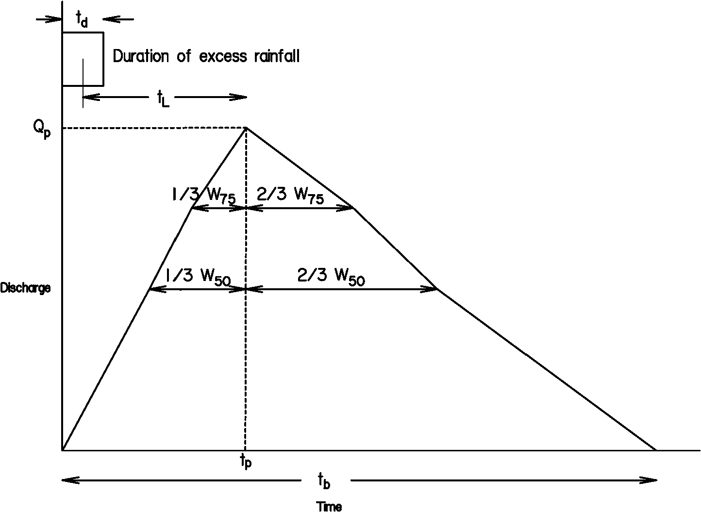
Figure 4-24. Snyder’s unit hydrograph
Values for W
50
and W75
are computed using these equations (McCuen 1989):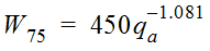
Equation 4-50.
Equation 4-51.
Where:
q
= peak discharge per square mile (i.e., Qa
p
/A, ft3
/sec/mi2
)