Reservoir Versus Channel Routing
Inflow hydrographs can be routed through reservoirs using a simple (single reservoir) hydrologic routing method, such as the modified Puls storage method. This is because the relationship between storage and discharge is unique (single-valued). In other words, the storage in the reservoir is fully described by the stage in the reservoir because the surface of the reservoir is the same shape and slope during the rising and falling limbs of the hydrograph.
Hydrologic routing methods may also be used for channel routing. A channel does not have a single-valued storage-outflow curve. Instead, the storage-outflow relation is looped, as shown in Figure 4-29. As a result, a hydrologic routing method employing a single reservoir representation cannot be used.
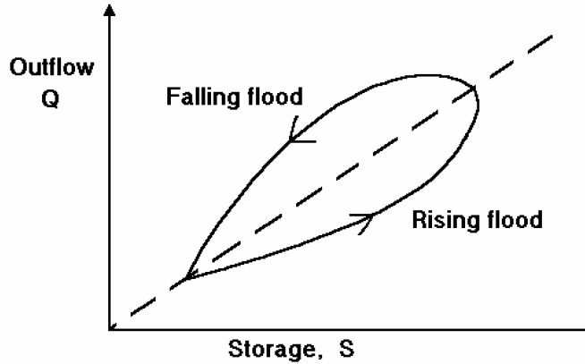
Figure 4-29. Looped storage outflow relation (USACE 1994)
The level-pool limitation of hydrologic routing methods is overcome by representing the channel as a series of reservoirs. These are termed subreaches, or steps, within the routing reach. Another enhancement to the level-pool approach, employed by the Muskingum method, is to represent the storage in each reservoir as a combination of prism storage (similar to level-pool reservoir) and wedge storage (additional sloped water on top of prism).
An estimate of the number of routing steps required for a hydrologic channel routing method is given by (USACE 1994):

Equation 4-66.
Where:
- n= number of routing steps
- K= floodwave travel time through the reach (min.)
- Dt= time step (min.)
K
in the above equation is given by:
Equation 4-67.
Where:
- L= length of routing reach (ft)
- V= flood wave velocity (ft/s)W
V
W
may be approximated as equal to the average channel velocity during the flood hydrograph. A better estimate of VW
is given by Seddon’s law applied to a cross section representative of the routing reach (USACE 1994):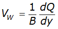
Equation 4-68.
Where:
- B= top with of the channel water surface (ft)
- Q= channel discharge (cfs) as function of elevation y
 = slope of the discharge rating curve (ft2/s)
Two hydrologic routing methods and their application are discussed further in the following sections: the modified Puls method for reservoir routing, and the Muskingum method for channel routing.
Modified Puls Method Reservoir Routing
Basic Concepts and Equations
The basic storage routing equation states that mass is conserved and can be expressed as follows: Average inflow - average outflow = Rate of change in storage
In numerical form, this statement of flow continuity can be written as:
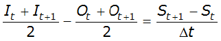
Equation 4-69.
Where:
- I= inflow at time step number tt
- I= inflow at time step number t + 1t+1
- O= outflow at time step number tt
- O= outflow at time step number t + 1t+1
- S= storage in the reservoir at time step number tt
- S= storage in the reservoir at time step number t + 1t+1
- Δt= the time increment
- Δt= the time increment *** REMOVE DUPLATE INFO IF DISPLAYS NICELY ***
- t= time step number
In Equation 4-64 there are two unknowns: O
t+1
and St+1
.
In order to solve Equation 4-64, either a second equation with Ot+1
and St+1
is required, or a relationship between Ot+1
and St+1
is needed.
The storage-indication approach is the latter and is presented here. First, it is convenient to rewrite the routing equation as: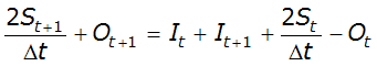
Equation 4-70.
In this form, all terms known at time t are on the right hand side of the equation and unknowns are on the left. If a single-valued storage-outflow curve can be determined for the routing reach, then for any value of O
t+1
, the corresponding value of S
t+1
will be known. This reduces the number of unknown parameters in Equation 4-65 from two (Ot+1
and St+1
) to one (Ot+1
).Use of the storage routing method requires the designer to determine the relationship between storage and outflow. This is simply the volume of water held by the reservoir, storage facility, or pond as a function of the water surface elevation or depth. For a reservoir or storage facility, this information is often available from the reservoir sponsor or owner.
For a pond or lake or where the stage-storage relation is not available, a relationship between storage and outflow can be derived from considerations of physical properties of channel or pond and simple hydraulic models of outlet works or relationship of flow and water surface elevation. These physical properties include:
- Ratings of the primary and/or emergency spillway of a reservoir.
- Pump flow characteristics in a pump station.
- Hydraulic performance curve of a culvert or bridge on a highway.
- Hydraulic performance curve of a weir and orifice outlet of a detention pond.
With the stage-storage relation established, a storage indication curve corresponding to the left side of Equation 4-68 is developed. The relationship is described in the form of O versus (2S/ΔT) + O. An example of a storage indication curve is provided in Figure 4-30.
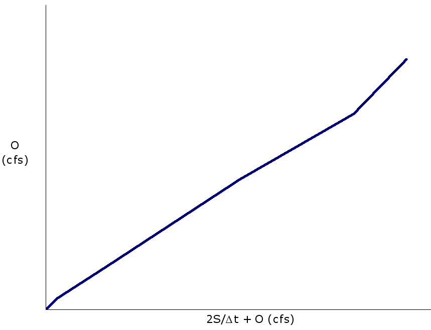
Figure 4-30. Sample storage-indication relation
The form of Equation 4-68 shown above is useful because the terms on the left side of the equation are known. With the relation between the outflow and storage determined (Figure 4-30), the ordinates on the outflow hydrograph can be determined directly.
Storage Routing Procedure
Use the following steps to route an inflow flood runoff hydrograph through a storage system such as a reservoir or detention pond:
- Acquire or develop a design flood runoff hydrograph for the project site watershed.
- Acquire or develop a stage-storage relation.
- Acquire or develop a stage-outflow relationship.
- Develop a storage-outflow relationship.
- Assume an initial value for Otas equal to It. At time step one (t = 1), assume an initial value for Otas equal to It. Usually, at time step one, inflow equals zero, so outflow will be zero and 2S1/ΔT - O1equals zero. Note that to start, t + 1 in the next step is 2.
- Compute 2St+1/ΔT + Ot+1using Equation 4-68.
- Interpolate to find the value of outflow. From the storage-outflow relation, interpolate to find the value of outflow (Ot+1) at (2St+1)/(ΔT)+Ot+1from step 6.
- Determine the value of (2St+1)/(ΔT)-Ot+1. Use the relation (2St+1)/(ΔT)-Ot+1= (2St+1)/(ΔT)+Ot+1- 2Ot+1.
- Assign the next time step to the value of t, e.g., for the first run through set t = 2.
- Repeat steps 6 through 9 until the outflow value (Ot+1) approaches zero.
- Plot the inflow and outflow hydrographs. The peak outflow value should always coincide with a point on the receding limb of the inflow hydrograph.
- Check conservation of mass to help verify success of the process. Use Equation 4-69 to compare the inflow volume to the sum of retained and outflow volumes:
 Equation 4-71.
Where:
- S= difference in starting and ending storage (ftr3or m3)
- SI= sum of inflow hydrograph ordinates (cfs or mt3/s)
- SO= sum of outflow hydrograph ordinates (cfs or mt3/s)
Muskingum Method Channel Routing
Routing of flood hydrographs by means of channel routing procedures is useful in instances where computed hydrographs are at points other than the points of interest. This is also true in those instances where the channel profile or plan is changed in such a way as to alter the natural velocity or channel storage characteristics. Routing estimates the effect of a channel reach on an inflow hydrograph. This section describes the Muskingum method equations, a lumped flow routing technique that approximates storage effects in the form of a prism and wedge component (Chow 1988).
The Muskingum method also solves the equation of continuity. With the Muskingum method, the storage in the channel is considered the sum of two components: prism storage and wedge storage (Figure 4-31).
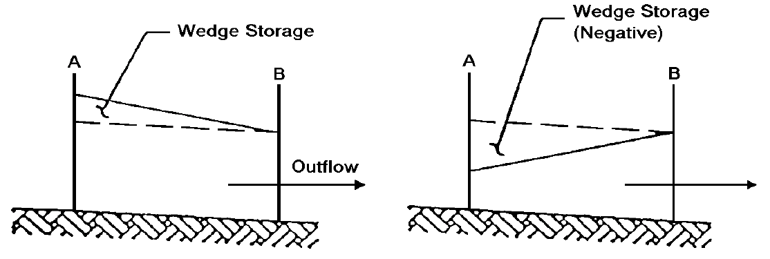
Figure 4-31. Muskingum prism and wedge storage
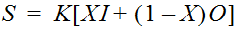
The constants K and X are used to relate the prism component, KO, and wedge component, KX(I-O), to the inflow and outflow of the reach:
Equation 4-72.
Where:
- S= total storage (ft3or m3)
- K= a proportionality constant representing the time of travel of a flood wave to traverse the reach (s). Often, this is set to the average travel time through the reach.
- X= a weighting factor describing the backwater storage effects approximated as a wedge
- I= inflow (cfs or m3/s)
- O= outflow (cfs or m3/s)
The value of X depends on the amount of wedge storage; when X = 0, there is no backwater (reservoir type storage), and when X = 0.5, the storage is described as a full wedge. The weighting factor, X, ranges from 0 to 0.3 in natural streams. A value of 0.2 is typical.
Equation 4-68 represents the time rate of change of storage as the following:
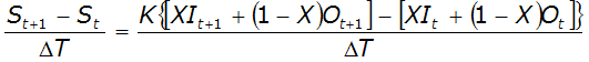
Equation 4-73.
Where:
- DT= time interval usually ranging from 0.3K to K
- t= time step number
Combining Equation 4-70 with Equation 4-71 yields the Muskingum flow routing equation:
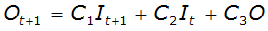
Equation 4-74.
Where:
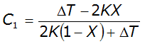
Equation 4-75.
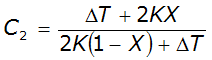
Equation 4-76.
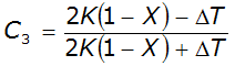
Equation 4-77.
By definition, the sum of C, C
1
2
, and C3
is 1. If measured inflow and outflow hydrographs are available, K and X can be estimated using Equation 4-71. Calculate X by plotting the numerator on the vertical axis and the denominator on the horizontal axis, and adjusting X until the loop collapses into a single line. The slope of the line equals K: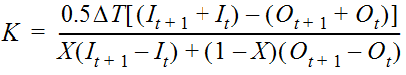
Equation 4-78.
The designer may also estimate K and X using the Muskingum-Cunge method described in Chow 1988 or Fread 1993.