Rainfall Temporal Distribution
The temporal rainfall distribution is how rainfall intensity varies over time for a single event. The mass rainfall curve, illustrated in Figure 4-13, is the cumulative precipitation up to a specific time. In drainage design, the storm is divided into time increments, and the average depth during each time increment is estimated, resulting in a rainfall hyetograph as shown in Figure 4-14.
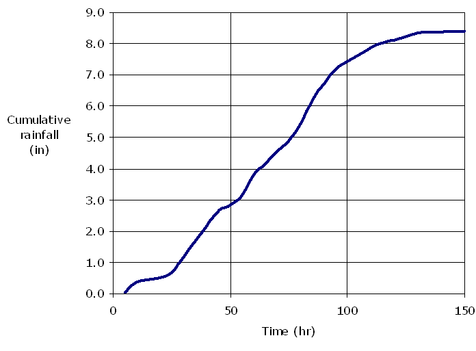
Figure 4-13. Example mass rainfall curve from historical storm
Hyetograph Development Procedure
In the rational method, the intensity is considered to be uniform over the storm period. Hydrograph techniques, however, account for variability of the intensity throughout a storm. Therefore, when using hydrograph techniques, the designer must determine a rainfall hyetograph: a temporal distribution of the watershed rainfall, as shown in Figure 4-14.
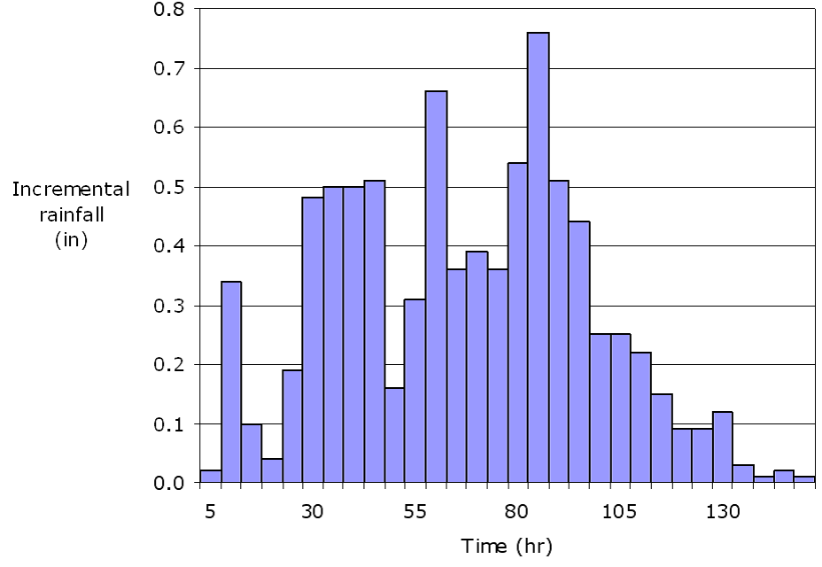
Figure 4-14. Rainfall hyetograph
Methods acceptable for developing a rainfall hyetograph for a design storm include the
method, the balanced storm method, and the Texas storm method.
NRCS Hyetograph Development Procedure
The NRCS design storm hyetographs were derived by averaging storm patterns for regions of the U.S. The storms thus represent a pattern distribution of rainfall over a 24-hour period to which a design rainfall depth can be applied. The distribution itself is arranged in a critical pattern with the maximum precipitation period occurring just before the midpoint of the storm.
The Natural Resources Conservation Service (NRCS) National Engineering Handbook (NEH), Part 630, Chapter 4 includes a detailed discussion on updating the temporal distribution of rainfall based on the new NOAA Atlas 14 rainfall data from the older NRCS Type II-III distributions commonly used in Texas, through 2019. TxDOT is evaluating whether to develop certain statewide temporal distribution zones similar to what Type II-III provided and further guidance may be forthcoming. Meanwhile, continued use of Type II and III temporal distribution of rainfall for Texas is no longer recommended, and the balanced storm method (also known as Frequency storm in HEC-HMS) is now preferred based on NRCS recommendations (NEH, Part 630.04).
Balanced Storm Hyetograph Development Procedure
The temporal distribution, with the peak of the storm located at the center of the hyetograph, is also called balanced storm. It uses DDF values that are based on a statistical analysis of historical data.
HEC-HMS software can derive hyetographs with the balanced method when the center of the storm is specified to be at 50% of the total storm duration. HEC-HMS also provides the ability to shift the peak from 50% of the total storm duration to 25%, 33%, 67%, or 75% as well, while maintaining the "nested" effect of the balanced storm.
The procedure for deriving a hyetograph with this method is as follows:
- For the selected , tabulate rainfall amounts for a storm of a given return period for all durations up to a specified limit (for 24-hour, 15-minute, 30-minute, 1-hour, 2-hour, 3-hour, 6-hour, 12-hour, 24-hour, etc.). Use for the duration and AEP selected for design.
- Select an appropriate time interval. An appropriate time interval is related to the time of concentration of the watershed. To calculate the time interval, use:
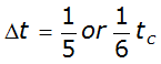 Equation 4-25.Where:
- Dt= time interval
- t= time of concentrationc
- For example, if the time of concentration is 1 hour, Δt = 1/5tc= 1/5 of 1 hour = 12 minutes, or 1/6 of 1 hour = 10 minutes. Choosing 1/5 or 1/6 will not make a significant difference in the distribution of the rainfall; use one fraction or the other to determine a convenient time interval.
- For successive times of interval Δt, find the cumulative rainfall depths from the DDF values. For depths at time intervals not included in the DDF tables, interpolate depths for intermediate durations using a log-log interpolation. (Durations from the table are usually given in hours, but in minutes on the plot.) For example, given a study area in the northern part of Bexar County, the log-log plot in Figure 4-15 shows the 10% depths for the 15-, 30-, 60-, 120-, 180-, 360-, 720-, and 1440-minute durations included in Asquith and Roussel 2004. The precipitation depth at 500 minutes is interpolated as 5.0 inches.
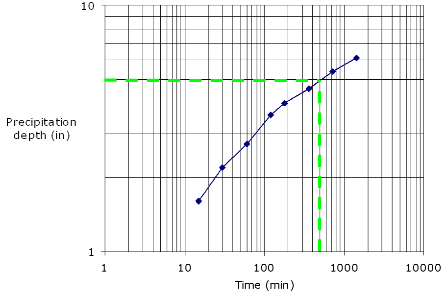 Figure 4-15. Log time versus log precipitation depth
 - Find the incremental depths by subtracting the cumulative depth at a particular time interval from the depth at the previous time interval.
- Rearrange the incremental depths so that the peak depth is at the center of the storm and the remaining incremental depths alternate (to left and right of peak) in descending order.
For example, in Figure 4-16, the largest incremental depth for a 24-hour storm (1,440 minutes) is placed at the 720-minute time interval and the remaining incremental depths are placed about the 720-minute interval in alternating decreasing order.
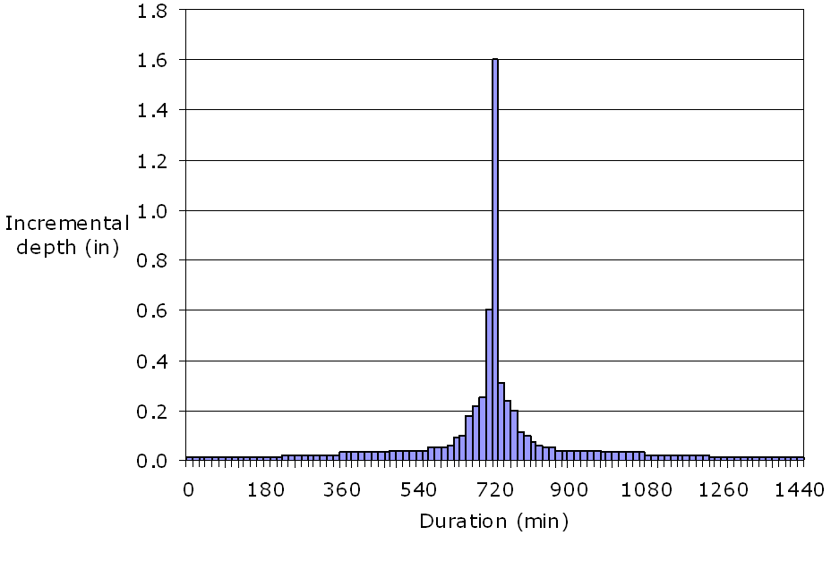
Figure 4-16. Balanced storm hyetograph