Models for Estimating Losses
Losses refer to the volume of rain falling on a watershed that does not run off. With each model, precipitation loss is found for each computation time interval, and is subtracted from the precipitation depth for that interval. The remaining depth is referred to as precipitation excess. This depth is considered uniformly distributed over a watershed area, so it represents a volume of runoff.
Loss models available to the TxDOT designer include:
- Initial and constant-rate loss model.
- Texas initial and constant-rate loss model.
- curve number loss model.
- Green and Ampt loss model.
Initial and Constant-Rate Loss Model
Basic Concepts and EquationsFor the initial loss and constant–rate loss model, no runoff occurs in the watershed until an initial loss capacity has been satisfied, regardless of the rainfall rate. Once the initial loss has been satisfied, a constant potential loss rate occurs for the duration of the storm. This method is a simple approximation of a typical infiltration curve, where the initial loss decays over the storm duration to a final near-constant loss rate. In the example in Figure 4-19, the initial loss is satisfied in the first time increment, and the constant rate accounts for losses thereafter.
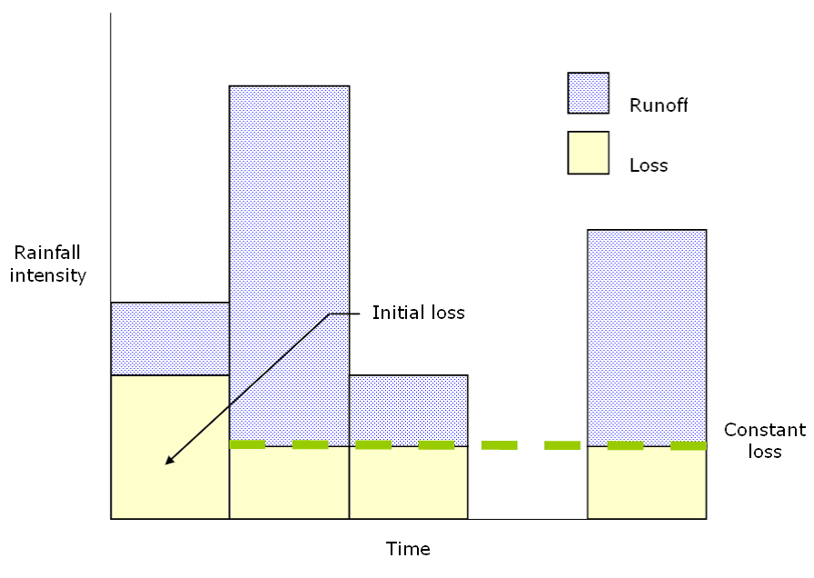
Figure 4-19. Initial and constant-loss rate model
The initial and constant loss-rate model is described mathematically as:
Equation 4-29.

Equation 4-30.

Equation 4-31.
Where:
- I(t)= rainfall intensity (in./hr.)
- f(t)= loss rate (in./hr.)
- P(t)= cumulative rainfall depth (in.) at time t
- I= initial loss (in.)a
- L= constant loss rate (in./hr.)
I
a
accounts for interception and depression storage, and the initial rate of infiltration at the beginning of the storm event. Interception refers to the capture of rainfall on the leaves and stems of vegetation before it reaches the ground surface. Depression storage is where the ponded rainfall fills small depressions and irregularities in the ground surface. Depression storage eventually infiltrates or evaporates during dry-weather periods. Until the accumulated precipitation on the pervious area exceeds the initial loss volume, no runoff occurs.Estimating Initial Loss and Constant Rate
The initial and constant-rate loss model includes one parameter (the constant rate) and one initial condition (the initial loss). Respectively, these represent physical properties of the watershed soils and land use and the antecedent condition.
If the watershed is in a saturated state, I
a
will approach 0. If the watershed is dry, then Ia
will increase to represent the maximum precipitation depth that can fall on the watershed with no runoff; this will depend on the watershed terrain, land use, soil types, and soil treatment.The constant loss rate can be viewed as the ultimate infiltration capacity of the soils. The
classified soils on the basis of this infiltration capacity as presented in Table 4-17; values in Column 4 represent reasonable estimates of the rates.
Texas Initial and Constant-Rate Loss Model
Recent research (TxDOT 0-4193-7) developed four computational approaches for estimating initial abstraction (I
A
) and constant loss (CL
) values for watersheds in Texas. The approaches are all based on the analysis of rainfall and runoff data of 92 gauged watersheds in Texas. One of those methods, presented here, allows the designer to compute IA
and CL
from regression equations:
Equation 4-32.

Equation 4-33.
Where:
- I= initial abstraction (in.)A
- C= constant loss rate (in./hr.)L
- L= main channel length (mi.)
- D= 0 for undeveloped watersheds, 1 for developed watersheds
- R= 0 for non-rocky watersheds, 1 for rocky watersheds
- CN= NRCS curve number
In the above equations, L is defined as “the length in stream-course miles of the longest defined channel shown in a 30-meter digital elevation model from the approximate watershed headwaters to the outlet” (TxDOT 0-4193-7).