NRCS Curve Number Loss Model
has developed a procedure to divide total depth of rainfall into soil retention, initial abstractions, and effective rainfall. This parameter is referred to as a curve number (CN). The CN is based on soil type, land use, and vegetative cover of the watershed. The maximum possible soil retention is estimated using a parameter that represents the impermeability of the land in a watershed. Theoretically, CN can range from 0 (100% rainfall infiltration) to 100 (impervious). In practice, based on values tabulated in NRCS 1986, the lowest CN the designer will likely encounter is 30, and the maximum CN is 98.
The CN may also be adjusted to account for wet or dry antecedent moisture conditions. Dry soil conditions are referred to as CN I, average conditions (those calculated using Estimating the CN) are referred to as CN II, and wet soils are referred to as CN III. Antecedent moisture conditions should be estimated considering a minimum of a five-day period. Antecedent soil moisture conditions also vary during a storm; heavy rain falling on a dry soil can change the soil moisture condition from dry to average to wet during the storm period.
Equation 4-34.
Equation 4-35.
Hydrologic Soil Groups
Soil properties influence the relationship between rainfall and runoff by affecting the rate of infiltration. NRCS divides soils into four hydrologic soil groups based on infiltration rates (Groups A-D). Urbanization has an effect on soil groups, as well. See Table 4-17 for more information.
Soil group | Description | Soil type | Range of loss rates | |
|---|---|---|---|---|
(in./hr.) | (mm/hr.) | |||
A | Low runoff potential due to high infiltration rates even when saturated | Deep sand, deep loess, aggregated silts | 0.30-0.45 | 7.6-11.4 |
B | Moderately low runoff potential due to moderate infiltration rates when saturated | Shallow loess, sandy loam | 0.15-0.30 | 3.8-7.6 |
C | Moderately high runoff potential due to slow infiltration rates Soils in which a layer near the surface impedes the downward movement of water or soils with moderately fine to fine texture | Clay loams, shallow sandy loam, soils low in organic content, and soils usually high in clay | 0.05-0.15 | 1.3-3.8 |
D | High runoff potential due to very slow infiltration rates | Soils that swell significantly when wet, heavy plastic clays, and certain saline soils | 0.00-0.05 | 1.3 |
Estimating the CN
Rainfall infiltration losses depend primarily on soil characteristics and land use (surface cover). The NRCS method uses a combination of soil conditions and land use to assign runoff CNs. Suggested runoff curve numbers are provided in Table 4-18, Table 4-19, Table 4-20, and Table 4-21. Note that CNs are whole numbers.
For a watershed that has variability in land cover and soil type, a composite CN is calculated and weighted by area.
Cover type and hydrologic condition | Average percent impervious area | A | B | C | D |
|---|---|---|---|---|---|
Open space (lawns, parks, golf courses, cemeteries, etc.): | |||||
Poor condition (grass cover < 50%) | 68 | 79 | 86 | 89 | |
Fair condition (grass cover 50% to 75%) | 49 | 69 | 79 | 84 | |
Good condition (grass cover > 75%) | 39 | 61 | 74 | 80 | |
Paved parking lots, roofs, driveways, etc. (excluding right-of-way) | 98 | 98 | 98 | 98 | |
Streets and roads: | |||||
Paved; curbs and storm drains (excluding right-of-way) | 98 | 98 | 98 | 98 | |
Paved; open ditches (including right-of-way) | 83 | 89 | 92 | 93 | |
Gravel (including right-of-way) | 76 | 85 | 89 | 91 | |
Dirt (including right-of-way) | 72 | 82 | 87 | 89 | |
Western desert urban areas: | |||||
Natural desert landscaping (pervious areas only) | 63 | 77 | 85 | 88 | |
Artificial desert landscaping (impervious weed barrier, desert shrub with 1- to 2-in. sand or gravel mulch and basin borders) | 96 | 96 | 96 | 96 | |
Urban districts: | |||||
Commercial and business | 85 | 89 | 92 | 94 | 95 |
Industrial | 72 | 81 | 88 | 91 | 93 |
Residential districts by average lot size: | |||||
1/8 acre or less (townhouses) | 65 | 77 | 85 | 90 | 92 |
1/4 acre | 38 | 61 | 75 | 83 | 87 |
1/3 acre | 30 | 57 | 72 | 81 | 86 |
1/2 acre | 25 | 54 | 70 | 80 | 85 |
1 acre | 20 | 51 | 68 | 79 | 84 |
2 acres | 12 | 46 | 65 | 77 | 82 |
Developing urban areas: Newly graded areas (pervious area only, no vegetation) | 77 | 86 | 91 | 94 | |
Notes: Values are for average runoff condition, and I a = 0.2S. The average percent impervious area shown was used to develop the composite CNs. Other assumptions are: impervious areas are directly connected to the drainage system, impervious areas have a CN of 98, and pervious areas are considered equivalent to open space in good hydrologic condition. | |||||
Cover type | Treatment | Hydrologic condition | A | B | C | D |
|---|---|---|---|---|---|---|
Fallow | Bare soil | - | 77 | 86 | 91 | 94 |
Crop residue cover (CR) | Poor Good | 76 74 | 85 83 | 90 88 | 93 90 | |
Row crops | Straight row (SR) | Poor Good | 72 67 | 81 78 | 88 85 | 91 89 |
SR + CR | Poor Good | 71 64 | 80 75 | 87 82 | 90 85 | |
Contoured (C) | Poor Good | 70 65 | 79 75 | 84 82 | 88 86 | |
C + CR | Poor Good | 69 64 | 78 74 | 83 81 | 87 85 | |
Contoured & terraced (C&T) | Poor Good | 66 62 | 74 71 | 80 78 | 82 81 | |
C&T + CR | Poor Good | 65 61 | 73 70 | 79 77 | 81 80 | |
Small grain | SR | Poor Good | 65 63 | 76 75 | 84 83 | 88 87 |
SR + CR | Poor Good | 64 60 | 75 72 | 83 80 | 86 84 | |
C | Poor Good | 63 61 | 74 73 | 82 81 | 85 84 | |
C + CR | Poor Good | 62 60 | 73 72 | 81 80 | 84 83 | |
C&T | Poor Good | 61 59 | 72 70 | 79 78 | 82 81 | |
C&T + CR | Poor Good | 60 58 | 71 69 | 78 77 | 81 80 | |
Close-seeded or broadcast legumes or rotation meadow | SR | Poor Good | 66 58 | 77 72 | 85 81 | 89 85 |
C | Poor Good | 64 55 | 75 69 | 83 78 | 85 83 | |
C&T | Poor Good | 63 51 | 73 67 | 80 76 | 83 80 | |
Notes: Values are for average runoff condition, and I a = 0.2S. Crop residue cover applies only if residue is on at least 5% of the surface throughout the year. Hydrologic condition is based on a combination of factors affecting infiltration and runoff: density and canopy of vegetative areas, amount of year-round cover, amount of grass or closed-seeded legumes in rotations, percent of residue cover on land surface (good > 20%), and degree of roughness. Poor = Factors impair infiltration and tend to increase runoff. Good = Factors encourage average and better infiltration and tend to decrease runoff. | ||||||
Cover type | Hydrologic condition | A | B | C | D |
|---|---|---|---|---|---|
Pasture, grassland, or range-continuous forage for grazing | Poor Fair Good | 68 49 39 | 79 69 61 | 86 79 74 | 89 84 80 |
Meadow – continuous grass, protected from grazing and generally mowed for hay | - | 30 | 58 | 71 | 78 |
Brush – brush-weed-grass mixture, with brush the major element | Poor Fair Good | 48 35 30 | 67 56 48 | 77 70 65 | 83 77 73 |
Woods – grass combination (orchard or tree farm) | Poor Fair Good | 57 43 32 | 73 65 58 | 82 76 72 | 86 82 79 |
Woods | Poor Fair Good | 45 36 30 | 66 60 55 | 77 73 70 | 83 79 77 |
Farmsteads – buildings, lanes, driveways, and surrounding lots | - | 59 | 74 | 82 | 86 |
Notes: Values are for average runoff condition, and I a = 0.2S. Pasture: Poor is < 50% ground cover or heavily grazed with no mulch, Fair is 50% to 75% ground cover and not heavily grazed, and Good is > 75% ground cover and lightly or only occasionally grazed. Meadow: Poor is < 50% ground cover, Fair is 50% to 75% ground cover, Good is > 75% ground cover. Woods/grass: CNs shown were computed for areas with 50 percent grass (pasture) cover. Other combinations of conditions may be computed from CNs for woods and pasture. Woods: Poor = forest litter, small trees, and brush destroyed by heavy grazing or regular burning. Fair = woods grazed but not burned and with some forest litter covering the soil. Good = woods protected from grazing and with litter and brush adequately covering soil. | |||||
Cover type | Hydrologic condition | A | B | C | D |
|---|---|---|---|---|---|
Herbaceous—mixture of grass, weeds, and low-growing brush, with brush the minor element | Poor Fair Good | 80 71 62 | 87 81 74 | 93 89 85 | |
Oak-aspen—mountain brush mixture of oak brush, aspen, mountain mahogany, bitter brush, maple, and other brush | Poor Fair Good | 66 48 30 | 74 57 41 | 79 63 48 | |
Pinyon-juniper—pinyon, juniper, or both; grass understory | Poor Fair Good | 75 58 41 | 85 73 61 | 89 80 71 | |
Sagebrush with grass understory | Poor Fair Good | 67 51 35 | 80 63 47 | 85 70 55 | |
Saltbush, greasewood, creosote-bush, blackbrush, bursage, palo verde, mesquite, and cactus | Poor Fair Good | 63 55 49 | 77 72 68 | 85 81 79 | 88 86 84 |
Notes: Values are for average runoff condition, and I a = 0.2S. Hydrologic Condition: Poor = < 30% ground cover (litter, grass, and brush overstory), Fair = 30% to 70% ground cover, Good = > 70% ground cover. Curve numbers for Group A have been developed only for desert shrub. | |||||
Soil Retention
The potential maximum retention (S) is calculated as:
Equation 4-36.
Where:
- z= 10 for English measurement units, or 254 for metric
- CN= runoff curve number
Equation 4-36 is valid if S is less than the rainfall excess, defined as precipitation (P) minus runoff (R) or S < (P-R). This equation was developed mainly for small watersheds from recorded storm data that included total rainfall amount in a calendar day but not its distribution with respect to time. Therefore, this method is appropriate for estimating direct runoff from 24-hour or 1-day storm rainfall.
Initial Abstraction
The initial abstraction consists of interception by vegetation, infiltration during early parts of the storm, and surface depression storage.
Generally, I
a
is estimated as:
Equation 4-37.
Effective Rainfall Runoff Volume
The effective rainfall (or the total rainfall minus the initial abstractions and retention) used for runoff hydrograph computations can be estimated using:
Equation 4-38.
Where:
- Pe= accumulated excess rainfall (in.)
- Ia= initial abstraction before ponding (in.)
- P = total depth of rainfall (in.)
- S = potential maximum depth of water retained in the watershed (in.)
Substituting Equation 4-37, Equation 4-38 becomes:
Equation 4-39.
P
e
and P have units of depth, Pe
and P reflect volumes and are often referred to as volumes because it is usually assumed that the same depths occurred over the entire watershed. Therefore Pe
is considered the volume of direct runoff per unit area, i.e., the rainfall that is neither retained on the surface nor infiltrated into the soil. Pe
also can be applied sequentially during a storm to compute incremental precipitation for selected time interval Δt.Climatic Adjustment of CN
NRCS curve numbers, estimated (predicted) using the procedure described in
Estimating the CN
, may be adjusted to account for the variation of climate within Texas. The adjustment is applied as follows:
Equation 4-40.
Where:
- CN= CN adjusted for climateobs
- CN= Estimated CN from NRCS procedures described inpredEstimating the CN
- CN= Deviation of CNdevobsfrom CNpred= climatic adjustment factor
In two studies (Hailey and McGill 1983, Thompson et al. 2003) CN
dev
was computed for gauged watersheds in Texas as CNobs
- CNpred
based on historical rainfall and runoff volumes. These studies show that CNdev
varies by location within the state.The following excerpt (Thompson et al. 2003) guides the designer in selection and application of the appropriate climatic adjustment to the predicted CN.
Given the differences between CN
obs
and CNpred
, it is possible to construct a general adjustment to CNpred
such that an approximation of CNobs
can be obtained. The large amount of variation in CNobs
does not lend to smooth contours or function fits. There is simply an insufficient amount of information for these types of approaches. However, a general adjustment can be implemented using regions with a general adjustment factor. Such an approach was taken and is presented in Figure 4-20.The bulk of rainfall and runoff data available for study were measured near the I-35 corridor. Therefore, estimates for this region are the most reliable. The greater the distance from the majority of the watershed that were part of this study, then the more uncertainty must be implied about the results. For the south high plains, that area south of the Balcones escarpment, and the coastal plain, there was insufficient data to make any general conclusions.
Application of the tool is straightforward. For areas where adjustment factors are defined (see Figure 4-20) the analyst should:
- Determine CNpredusing the normal NRCS procedure.
- Find the location of the watershed on the design aid (Figure 4-21). Determine an adjustment factor from the design aid and adjust the curve number.
- Examine Figure 4-21 and find the location of the watershed. Use the location of the watershed to determine nearby study watersheds. Then refer to Figure 4-20 and Table 4-22, Table 4-23, Table 4-24, Table 4-25, and Table 4-26 and determine CNpredand CNobsfor study watersheds near the site in question, if any are near the watershed in question.
- Compare the adjusted curve number with local values of CNobs.
The result should be a range of values that are reasonable for the particular site.
As a comparison, the adjusted curve number from Hailey and McGill (Figure 4-22) can be used.
A lower bound equivalent to the curve number for AMC I (dry antecedent conditions), or a curve number of 60, whichever is greater, should be considered.
Note that CN values are whole numbers. Rounding of values of CN
pred
in the tables may be required.Judgment is required for application of any hydrologic tool. The adjustments presented on Figure 4-20 are no exception. A lower limit of AMC I may be used to prevent an overadjustment downward. For areas that have few study watersheds, the Hailey and McGill approach should provide some guidance on the amount of reduction to CN
pred
is appropriate, if any.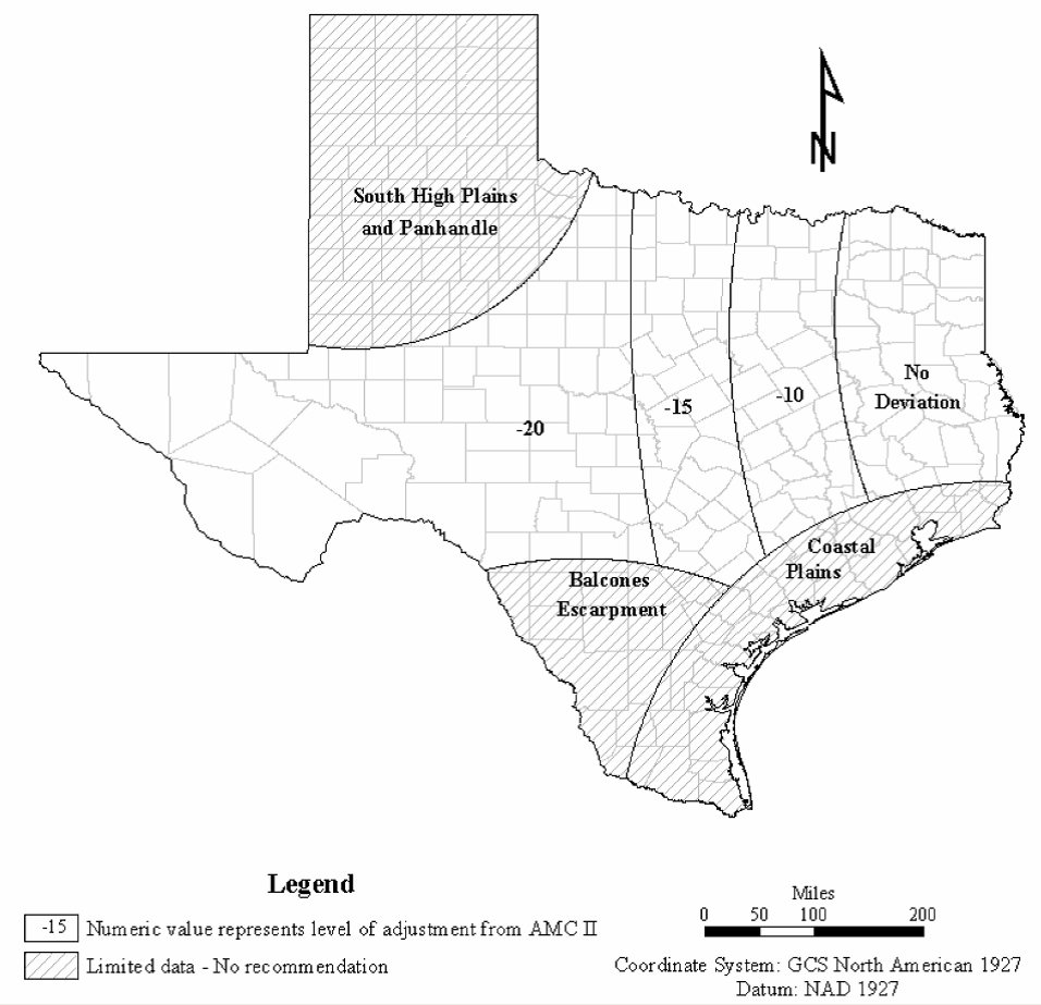
Figure 4-20. Climatic adjustment factor CN
dev
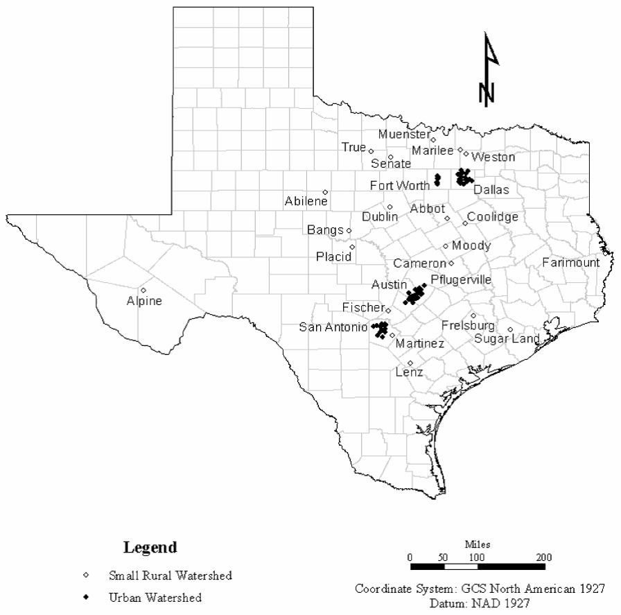
Figure 4-21. Location of CNdev watersheds
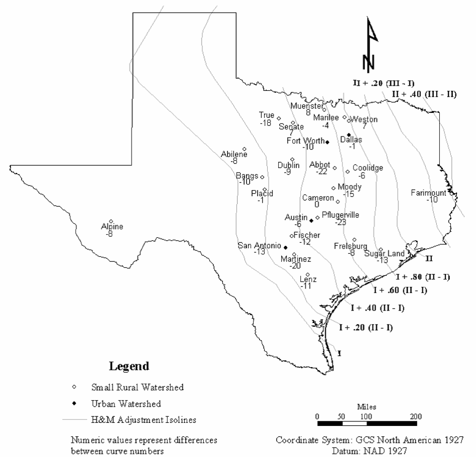
Climatic adjustment of CN - comparison of Hailey and McGill adjusted curve numbers, CNH&M, with CNobs. Negative differences indicate that CNH&M is larger than CNobs. Also shown are the lines of equal adjustment to curve number from Hailey and McGill’s (1983) Figure 4. (click in image to see full-size image)
USGS Gauge ID | Quad Sheet Name | CN obs | CN pred | CN dev |
|---|---|---|---|---|
8154700 | Austin West | 59 | 68.9 | -9.9 |
8155200 | Bee Cave | 65 | 70.7 | -5.7 |
8155300 | Oak Hill | 64 | 69.8 | -5.8 |
8155550 | Austin West | 50 | 87.3 | -37.3 |
8156650 | Austin East | 60 | 83.6 | -23.6 |
8156700 | Austin East | 78 | 86.6 | -8.6 |
8156750 | Austin East | 66 | 86.8 | -20.8 |
8156800 | Austin East | 66 | 87 | -21 |
8157000 | Austin East | 68 | 88.3 | -20.3 |
8157500 | Austin East | 67 | 89.1 | -22.1 |
8158050 | Austin East | 71 | 83.9 | -12.9 |
8158100 | Pflugerville West | 60 | 72.6 | -12.6 |
8158200 | Austin East | 62 | 75.6 | -13.6 |
8158400 | Austin East | 79 | 88.9 | -9.9 |
8158500 | Austin East | 71 | 85.6 | -14.6 |
8158600 | Austin East | 73 | 76.7 | -3.7 |
8158700 | Driftwood | 69 | 74.5 | -5.5 |
8158800 | Buda | 64 | 73.3 | -9.3 |
8158810 | Signal Hill | 64 | 69.8 | -5.8 |
8158820 | Oak Hill | 60 | 67.9 | -7.9 |
8158825 | Oak Hill | 49 | 67.2 | -18.2 |
8158840 | Signal Hill | 74 | 69.8 | 4.2 |
8158860 | Oak Hill | 60 | 68 | -8 |
8158880 | Oak Hill | 67 | 79.4 | -12.4 |
8158920 | Oak Hill | 71 | 77.5 | -6.5 |
8158930 | Oak Hill | 56 | 75.2 | -19.2 |
8158970 | Montopolis | 56 | 77.7 | -21.7 |
8159150 | Pflugerville East | 63 | 78.8 | -15.8 |
USGS Gauge ID | Quad Sheet Name | CN obs | CN pred | CN dev |
|---|---|---|---|---|
8055580 | Garland | 85 | 85.2 | -0.2 |
8055600 | Dallas | 82 | 86.1 | -4.1 |
8055700 | Dallas | 73 | 85.5 | -12.5 |
8056500 | Dallas | 85 | 85.8 | -0.8 |
8057020 | Dallas | 75 | 85.5 | -10.5 |
8057050 | Oak Cliff | 75 | 85.7 | -10.7 |
8057120 | Addison | 77 | 80.2 | -3.2 |
8057130 | Addison | 89 | 82.9 | 6.1 |
8057140 | Addison | 78 | 86.8 | -8.8 |
8057160 | Addison | 80 | 90.3 | -10.3 |
8057320 | White Rock Lake | 85 | 85.7 | -0.7 |
8057415 | Hutchins | 73 | 87.8 | -14.8 |
8057418 | Oak Cliff | 85 | 79.1 | 5.9 |
8057420 | Oak Cliff | 80 | 81 | -1 |
8057425 | Oak Cliff | 90 | 82.9 | 7.1 |
8057435 | Oak Cliff | 82 | 81.1 | 0.9 |
8057440 | Hutchins | 67 | 79.1 | -12.1 |
8057445 | Hutchins | 60 | 86.5 | -26.5 |
8061620 | Garland | 82 | 85 | -3 |
8061920 | Mesquite | 85 | 86 | -1 |
8061950 | Seagoville | 82 | 85.3 | -3.3 |
Gauge ID | Quad Sheet Name | CN obs | CN pred | CN dev |
|---|---|---|---|---|
8048520 | Fort Worth | 72 | 82.3 | -10.3 |
8048530 | Fort Worth | 69 | 86.7 | -17.7 |
8048540 | Covington | 73 | 88 | -15 |
8048550 | Haltom City | 74 | 91.2 | -17.2 |
8048600 | Haltom City | 65 | 84.3 | -19.3 |
8048820 | Haltom City | 67 | 83.4 | -16.4 |
8048850 | Haltom City | 72 | 83 | -11 |
USGS Gauge ID | Quad Sheet Name | CN obs | CN pred | CN dev |
|---|---|---|---|---|
8177600 | Castle Hills | 70 | 84.8 | -14.8 |
8178300 | San Antonio West | 72 | 85.7 | -13.7 |
8178555 | Southton | 75 | 84.2 | -9.2 |
8178600 | Camp Bullis | 60 | 79.7 | -19.7 |
8178640 | Longhorn | 56 | 78.4 | -22.4 |
8178645 | Longhorn | 59 | 78.2 | -19.2 |
8178690 | Longhorn | 78 | 84.4 | -6.4 |
8178736 | San Antonio East | 74 | 92.3 | -18.3 |
8181000 | Helotes | 50 | 79.2 | -29.2 |
8181400 | Helotes | 56 | 79.8 | -23.8 |
8181450 | San Antonio West | 60 | 87.3 | -27.3 |
USGS Gauge ID | Quadrangle Sheet Name | CN obs | CN pred | CN dev |
|---|---|---|---|---|
8025307 | Fairmount | 53 | 55.4 | -2.4 |
8083420 | Abilene East | 65 | 84.7 | -19.7 |
8088100 | True | 60 | 85.9 | -25.9 |
8093400 | Abbott | 61 | 88.1 | -27.1 |
8116400 | Sugarland | 70 | 82.9 | -12.9 |
8159150 | Pflugerville East | 55 | 83.7 | -28.7 |
8160800 | Freisburg | 56 | 67.8 | -11.8 |
8167600 | Fischer | 51 | 74.3 | -23.3 |
8436520 | Alpine South | 64 | 86.4 | -22.4 |
8435660 | Alpine South | 48 | 86.7 | -38.7 |
8098300 | Rosebud | 88 | 80.5 | 7.5 |
8108200 | Yarrelton | 77 | 79.9 | -2.9 |
8096800 | Bruceville | 62 | 80 | -18 |
8094000 | Bunyan | 60 | 78.4 | -18.4 |
8136900 | Bangs West | 51 | 75.8 | -24.8 |
8137000 | Bangs West | 52 | 74.5 | -22.5 |
8137500 | Trickham | 53 | 76.5 | -23.5 |
8139000 | Placid | 53 | 74.6 | -21.6 |
8140000 | Mercury | 63 | 74.4 | -11.4 |
8182400 | Martinez | 52 | 80 | -28 |
8187000 | Lenz | 53 | 83.8 | -30.8 |
8187900 | Kenedy | 63 | 73.3 | -10.3 |
8050200 | Freemound | 80 | 79.6 | 0.4 |
8057500 | Weston | 80 | 78.2 | 1.8 |
8058000 | Weston | 86 | 80.1 | 5.9 |
8052630 | Marilee | 80 | 85.4 | -5.4 |
8052700 | Aubrey | 74 | 84.1 | -10.1 |
8042650 | Senate | 59 | 63.4 | -4.4 |
8042700 | Lynn Creek | 50 | 62.5 | -12.5 |
8042700 | Senate | 56 | 62 | -6 |
8042700 | Senate | 65 | 55.9 | 9.1 |
8063200 | Coolidge | 70 | 79.4 | -9.4 |