NRCS Dimensionless Unit Hydrograph
The
unit hydrograph model is based upon an analysis and averaging of a large number of natural unit hydrographs from a broad cross section of geographic locations and hydrologic regions. For convenience, the hydrograph is dimensionless, with discharge ordinates (Q
u
) divided by the peak discharge (Qp
) and the time values (t) divided by the time to peak (tp
).The time-base of the dimensionless unit hydrograph is approximately five times the time to peak, and approximately 3/8 of the total volume occurs before the time to peak. The inflection point on the recession limb occurs at 1.67 times the time to peak, and the hydrograph has a curvilinear shape. The curvilinear hydrograph can be approximated by a triangular hydrograph with similar characteristics.
The curvilinear dimensionless NRCS unit hydrograph is shown in Figure 4-25.
Figure 4-25. NRCS dimensionless unit hydrograph
The ordinates of the dimensionless unit hydrograph are provided in Table 4-29.
t/t p | Q/Q p |
|---|---|
0.0 | 0.00 |
0.1 | 0.03 |
0.2 | 0.10 |
0.3 | 0.19 |
0.4 | 0.31 |
0.5 | 0.47 |
0.6 | 0.66 |
0.7 | 0.82 |
0.8 | 0.93 |
0.9 | 0.99 |
1.0 | 1.00 |
1.1 | 0.99 |
1.2 | 0.93 |
1.3 | 0.86 |
1.4 | 0.78 |
1.5 | 0.68 |
1.6 | 0.56 |
1.7 | 0.46 |
1.8 | 0.39 |
1.9 | 0.33 |
2.0 | 0.28 |
2.2 | 0.207 |
2.4 | 0.147 |
2.6 | 0.107 |
2.8 | 0.077 |
3.0 | 0.055 |
3.2 | 0.04 |
3.4 | 0.029 |
3.6 | 0.021 |
3.8 | 0.015 |
4.0 | 0.011 |
4.5 | 0.005 |
5.0 | 0.00 |
Notes: Variables are defined as follows: t = time (min.); t p = time to peak of unit hydrograph (min.);Q = discharge (cfs); and Q p = peak discharge of unit hydrograph (cfs). | |
The following procedure assumes the area or subarea is reasonably homogeneous. That is, the watershed is subdivided into homogeneous areas. The procedure results in a hydrograph only from the direct uncontrolled area. If the watershed has been subdivided, it might be necessary to perform hydrograph channel routing, storage routing, and hydrograph superposition to determine the hydrograph at the outlet of the watershed.
Application of the
dimensionless unit hydrograph to a watershed produces a site-specific unit hydrograph model with which storm runoff can be computed. To do this, the basin lag time must be estimated. The time to peak of the unit hydrograph is related to the lag time by:
Equation 4-52.
Where:
- t= time to peak of unit hydrograph (min.)p
- t= basin lag time (min.)L
- Dt= the time interval of the unit hydrograph (min.)
This time interval must be the same as the Δt chosen for the design storm.
The time interval may be calculated by:
Equation 4-53.
And the lag time is calculated by:
Equation 4-54.
The peak discharge of the unit hydrograph is calculated by:
Equation 4-55.
Where:
- Q= peak discharge (cfs)p
- C= conversion factor (645.33)f
- K= 0.75 (constant based on geometric shape of dimensionless unit hydrograph)
- A= drainage area (mi2); and
- t= time to peak (hr.)p
Equation 4-55 can be simplified to:
Equation 4-56.
The constant 484, or peak rate
factor (PRF)
, defines a unit hydrograph with 3/8 of its area under the rising limb. As the watershed slope becomes very steep (mountainous), the constant in Equation 4-56 can approach a value of approximately 600. For flat, swampy areas, the constant may decrease to a value 100 or lower (210-VI-NEH, March 2007)
. For applications in Texas, the use of the constant 484 is recommended as a starting point, but adjustments to a different value may be warranted. Limited sources are available for guidance on PRF adjustments. One source, while developed for the southeast US, provides practical guidance based on watershed size and slope (Sheridan, 2002). Any adjustments to the PRF must be well documented in the drainage report and model notes.
After t
p
and Qp
are estimated using Equations 4-52 and 4-56, the site specific unit hydrograph may be developed by scaling the dimensionless unit hydrograph.For each time step of the analysis, the site specific unit hydrograph ordinates are multiplied by the excess rainfall depth. The resulting hydrograph are summed to produce the total runoff hydrograph for the watershed. This process is shown graphically in Figure 4-23. While the computations can be completed using a spreadsheet model, a manual convolution can be somewhat time-consuming. These computations are typically performed by hydrologic computer programs.
For example, assume an area of 240 acres (0.375 sq. mi.) with T= 9 min, t
c
of 1.12 hours and CN of 80. For 1 inch of excess rainfall, △t
p
= 45 min, and Qp
= 243 cfs, using Equations 4-53, 4-52 and 4-56 respectively.Column 1 of Table 4-30 shows the time interval of 9 minutes. Column 2 is calculated by dividing the time interval by t
p
, in this case 45 minutes. Values in Column 3 are found by using the t/tp
value in Column 2 to find the associated Qu
/Qp
value from the dimensionless unit hydrograph shown in Figure 4-25, interpolating if necessary. Column 4 is calculated by multiplying Column 3 by Qp
, in this case 243 cfs.Table 4-30: Example Site-specific Unit Hydrograph
t (min.) | t/t p | Q u /Qp | Q u (cfs) |
|---|---|---|---|
0 | 0.00 | 0.000 | 0 |
9 | 0.20 | 0.100 | 24 |
18 | 0.40 | 0.310 | 75 |
27 | 0.60 | 0.660 | 160 |
36 | 0.80 | 0.930 | 226 |
45 | 1.00 | 1.000 | 243 |
54 | 1.20 | 0.930 | 226 |
63 | 1.40 | 0.780 | 190 |
72 | 1.60 | 0.560 | 136 |
81 | 1.80 | 0.390 | 95 |
90 | 2.00 | 0.280 | 68 |
99 | 2.20 | 0.207 | 50 |
108 | 2.40 | 0.147 | 36 |
117 | 2.60 | 0.107 | 26 |
126 | 2.80 | 0.077 | 19 |
135 | 3.00 | 0.055 | 13 |
144 | 3.20 | 0.040 | 10 |
153 | 3.40 | 0.023 | 6 |
162 | 3.60 | 0.021 | 5 |
171 | 3.80 | 0.015 | 4 |
180 | 4.00 | 0.011 | 3 |
189 | 4.20 | 0.009 | 2 |
198 | 4.40 | 0.006 | 2 |
207 | 4.60 | 0.004 | 1 |
216 | 4.80 | 0.002 | 0 |
225 | 5.00 | 0 | 0 |
The example site-specific unit hydrograph is shown in Figure 4-26.
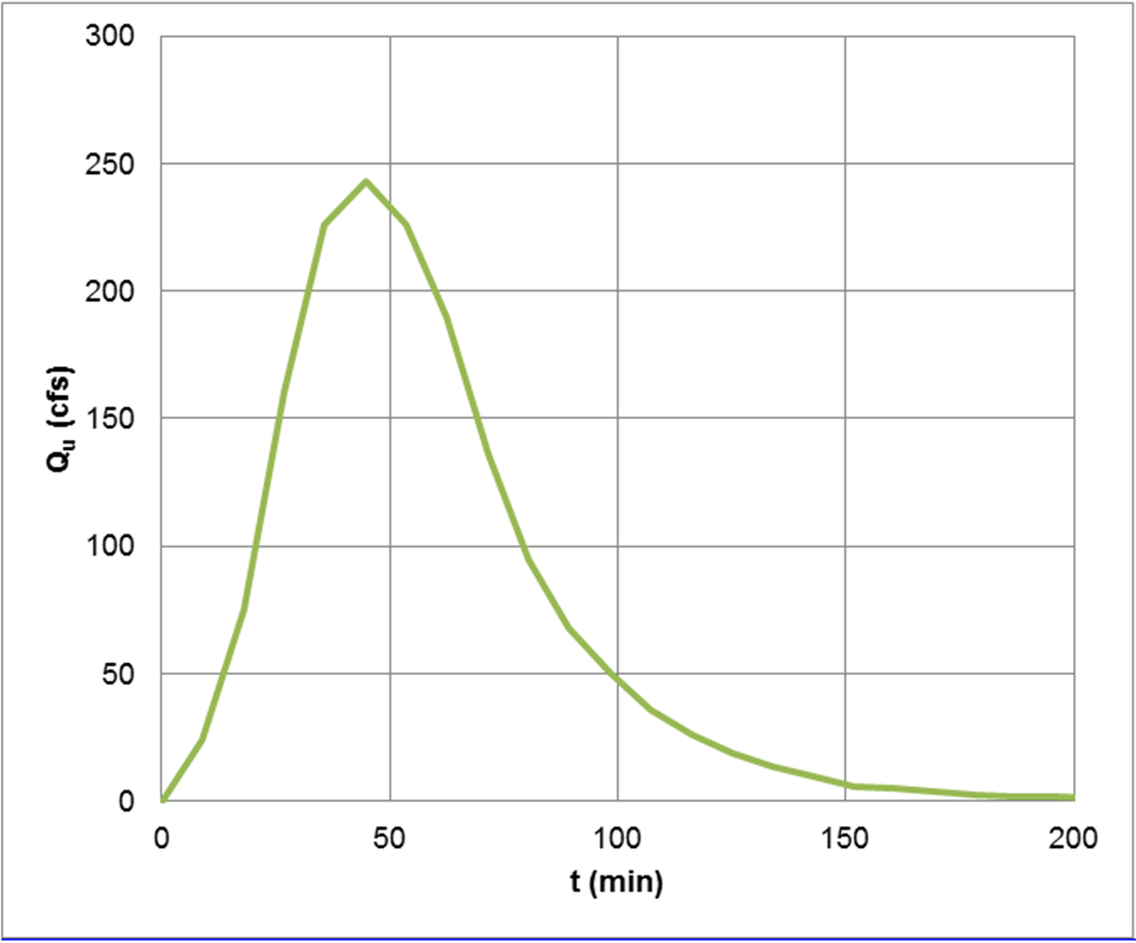
Figure 4-26. Example site-specific unit hydrograph
Remember that the site-specific hydrograph developed in Figure 4-26 was based on 1 inch of excess rainfall. For each time step of the analysis, the unit hydrograph ordinates are multiplied by the excess rainfall depth. Excess rainfall is obtained from a rainfall hyetograph such as a distribution developed from locally observed rainfall or the NRCS 24-hour, Type II or Type III rainfall distributions. The resulting hydrograph are summed to produce the total runoff hydrograph for the watershed. This process is shown graphically in Figure 4-24.
The capabilities and limitations of the NRCS unit hydrograph model include the following:
- This method does not account for variation in rainfall intensity or duration over the watershed.
- Baseflow is accounted for separately.