Section 3: Hydraulic Operation of Culverts
Parameters
The hydraulic operation and performance of a culvert involve a number of factors. You must determine, estimate, or calculate each factor as part of the hydraulic design or analysis.
The following procedures assume steady flow but can involve extensive calculations that lend themselves to computer application. The procedures supersede simplified hand methods of other manuals. TxDOT recommends computer models for all final design applications, although hand methods and nomographs may be used for initial planning.
Headwater under Inlet Control
Inlet control occurs when the culvert barrel is capable of conveying more flow than the inlet will accept. Inlet control is possible when the culvert slope is hydraulically steep (d
c
> du
). The control section of a culvert operating under inlet control is located just inside the entrance. When the flow in the barrel is free surface flow, critical depth occurs at or near this location, and the flow regime immediately downstream is supercritical. Depending on conditions downstream of the culvert inlet, a hydraulic jump may occur in the culvert. Under inlet control, hydraulic characteristics downstream of the inlet control section do not affect the culvert capacity. Upstream water surface elevation and inlet geometry (barrel shape, cross-sectional area, and inlet edge) are the major flow controls.A fifth-degree polynomial equation based on regression analysis is used to model the inlet control headwater for a given flow. Analytical equations based on minimum energy principles are matched to the regression equations to model flows that create inlet control heads outside of the regression data range. Equation 8-4 only applies when 0.5 ≤ HW
ic
/D ≤ 3.0.
Equation 8-4.
where:
- HWic= inlet control headwater (ft. or m)
- D= rise of the culvert barrel (ft. or m)
- S= culvert slope (ft./ft. or m/m)0
- F= function of average outflow discharge routed through a culvert; culvert barrel rise; and for box and pipe-arch culverts, width of the barrel, B, shown in Equation 8-5.
Equation 8-5.
where:
- W= width or span of culvert (ft. or m).
Shape and Material | Entrance Type | a | b | c | d | e | f |
RCP | Square edge w/headwall | 0.087483 | 0.706578 | -0.2533 | 0.0667 | -0.00662 | 0.000251 |
- | Groove end w/headwall | 0.114099 | 0.653562 | -0.2336 | 0.059772 | -0.00616 | 0.000243 |
- | Groove end projecting | 0.108786 | 0.662381 | -0.2338 | 0.057959 | -0.00558 | 0.000205 |
- | Beveled ring | 0.063343 | 0.766512 | -0.316097 | 0.08767 | -0.00984 | 0.000417 |
- | Improved (flared) inlet | 0.2115 | 0.3927 | -0.0414 | 0.0042 | -0.0003 | -0.00003 |
CMP | Headwall | 0.167433 | 0.53859 | -0.14937 | 0.039154 | -0.00344 | 0.000116 |
- | Mitered | 0.107137 | 0.757789 | -0.3615 | 0.123393 | -0.01606 | 0.000767 |
- | Projecting | 0.187321 | 0.567719 | -0.15654 | 0.044505 | -0.00344 | 0.00009 |
- | Improved (flared) inlet | 0.2252 | 0.3471 | -0.0252 | 0.0011 | -0.0005 | -0.00003 |
Box | 30-70º flared wingwall | 0.072493 | 0.507087 | -0.11747 | 0.02217 | -0.00149 | 0.000038 |
- | Parallel to 15º wingwall | 0.122117 | 0.505435 | -0.10856 | 0.020781 | -0.00137 | 0.0000346 |
- | Straight wingwall | 0.144138 | 0.461363 | -0.09215 | 0.020003 | -0.00136 | 0.000036 |
- | 45º wingwall w/top bevel | 0.156609 | 0.398935 | -0.06404 | 0.011201 | -0.00064 | 0.000015 |
- | Parallel headwall w/bevel | 0.156609 | 0.398935 | -0.06404 | 0.011201 | -0.00064 | 0.000015 |
- | 30º skew w/chamfer edges | 0.122117 | 0.505435 | -0.10856 | 0.020781 | -0.00137 | 0.000034 |
- | 10-45º skew w/bevel edges | 0.089963 | 0.441247 | -0.07435 | 0.012732 | -0.00076 | 0.000018 |
Oval B>D | Square edge w/headwall | 0.13432 | 0.55951 | -0.1578 | 0.03967 | -0.0034 | 0.00011 |
- | Groove end w/headwall | 0.15067 | 0.50311 | -0.12068 | 0.02566 | -0.00189 | 0.00005 |
- | Groove end projecting | -0.03817 | 0.84684 | -0.32139 | 0.0755 | -0.00729 | 0.00027 |
Oval D>B | Square edge w/headwall | 0.13432 | 0.55951 | -0.1578 | 0.03967 | -0.0034 | 0.00011 |
- | Groove end w/headwall | 0.15067 | 0.50311 | -0.12068 | 0.02566 | -0.00189 | 0.00005 |
- | Groove end projecting | -0.03817 | 0.84684 | -0.32139 | 0.0755 | -0.00729 | 0.00027 |
CM Pipe arch | Headwall | 0.111261 | 0.610579 | -0.194937 | 0.051289 | -0.00481 | 0.000169 |
- | Mitered | 0.083301 | 0.795145 | -0.43408 | 0.163774 | -0.02491 | 0.001411 |
- | Projecting | 0.089053 | 0.712545 | -0.27092 | 0.792502 | -0.00798 | 0.000293 |
Struct plate Pipe arch | Projecting—corner plate (17.7 in. or 450 mm) | 0.089053 | 0.712545 | -0.27092 | 0.792502 | -0.00798 | 0.000293 |
- | Projecting—corner plate (30.7 in. or 780 mm) | 0.12263 | 0.4825 | -0.00002 | -0.04287 | 0.01454 | -0.00117 |
CM arch (flat bottom) | Parallel headwall | 0.111281 | 0.610579 | -0.1949 | 0.051289 | -0.00481 | 0.000169 |
- | Mitered | 0.083301 | 0.795145 | -0.43408 | 0.163774 | -0.02491 | 0.001411 |
- | Thin wall projecting | 0.089053 | 0.712545 | -0.27092 | 0.792502 | -0.00798 | 0.000293 |
For HW
i
/D > 3.0, Equation 8-6, an orifice equation, is used to estimate headwater:- Determine the potential head from the centroid of the culvert opening, which is approximated as the sum of the invert elevation and one half the rise of the culvert. The effective area, A, and orifice coefficient, C, are implicit.
- Determine the coefficient, k, by rearranging Equation 8-6 using the discharge that creates a HW/D ratio of 3 in the regression equation, Equation 8-7 (i.e., the upper limit of the ):
Equation 8-6.
where:
- HWi= inlet control headwater depth (ft. or m)
- Q= design discharge (cfs or m3/s)
- k= orifice equation constant
- D= rise of culvert (ft. or m).
 Equation 8-7.
where:
- Q= discharge (cfs or m3.03/s) at which HW/D = 3.
Generally for TxDOT designs, it is not considered efficient to design culverts for HW
i
/D < 0.5. However, if such a condition is likely, an open channel flow minimum energy equation (weir equation) should be used, with the addition of a velocity head loss coefficient. The minimum energy equation, with the velocity head loss adjusted by an entrance loss coefficient, generally describes the low flow portion of the inlet control headwater curve. However, numerical errors in the calculation of flow for very small depths tend to increase the velocity head as the flow approaches zero. This presents little or no problem in most single system cases because the flows that cause this are relatively small.In many of the required calculations for the solution of multiple culverts, the inlet control curve must decrease continuously to zero for the iterative calculations to converge. Therefore, computer models modify this equation to force the velocity head to continually decrease to zero as the flow approaches zero.
The “Charts” in
(FHWA, Hydraulic Design of Highway Culverts) provide guidance for graphical solution of headwater under inlet control.
Headwater under Outlet Control
Outlet control occurs when the culvert barrel is not capable of conveying as much flow as the inlet opening will accept. Outlet control is likely only when the hydraulic grade line inside the culvert at the entrance exceeds critical depth. (See Chapter 6 for Hydraulic Grade Line Analysis.) Therefore, outlet control is most likely when the culvert is on a mild slope (d
n
> dc
). It is also possible to experience outlet control with a culvert on a steep slope (dn
< dc
) with a high tailwater such that subcritical flow or full flow exists in the culvert.The headwater of a culvert in outlet control is a function of discharge, conduit section geometry, conduit roughness characteristics, length of the conduit, profile of the conduit, entrance geometry (to a minor extent), and (possibly) tailwater level.
The headwater of a culvert under outlet control can be adjusted, for practical purposes, by modifying culvert size, shape, and roughness. Both inlet control and outlet control need to be considered to determine the headwater. The following table provides a summary conditions likely to control the culvert headwater. Refer to Figure 8‑4 and Figure 8‑5 to identify the appropriate procedures to make the determination.
Description | Likely Condition |
|---|---|
Hydraulically steep slope, backwater does not submerge critical depth at inside of inlet | Inlet control |
Hydraulically steep slope, backwater submerges critical depth at inside of inlet | Outlet control |
Hydraulically steep slope, backwater close to critical depth at inlet | Oscillate between inlet and outlet control. |
Hydraulically mild slope | Outlet control |
Outlet control headwater is determined by accounting for the total energy losses that occur from the culvert outlet to the culvert inlet. Figure 8‑7 and Figure 8‑8 and associated procedures in Section 4 should be used to analyze or design a culvert.
Outlet control headwater HW
oc
depth (measured from the flowline of the entrance) is expressed in terms of balancing energy between the culvert exit and the culvert entrance as indicated by Equation 8-8.
Equation 8-8.
where:
- HWoc= headwater depth due to outlet control (ft. or m)
- h= velocity head of flow approaching the culvert entrance (ft. or m)va
- h= velocity head in the entrance (ft. or m) as calculated using Equation 8-9.vi
- h= entrance head loss (ft. or m) as calculated usinge
- h= friction head losses (ft. or m) as calculated usingf
- S= culvert slope (ft./ft. or m/m)o
- L= culvert length (ft. or m)
- Ho= depth of hydraulic grade line just inside the culvert at outlet (ft. or m) (outlet depth).
 Equation 8-9.where:
 - v= flow velocity in culvert (ft./s or m/s).
- g= the gravitational acceleration = 32.2 ft/ s2or 9.81 m/s2.
For convenience energy balance at outlet, energy losses through barrel, and energy balance at inlet should be considered when determining outlet control headwater.
When the tailwater controls the outlet flow, Equation 8-10 represents the energy balance equation at the conduit outlet. Traditional practice has been to ignore exit losses. If exit losses are ignored, the hydraulic grade line inside the conduit at the outlet,outlet depth, H
o
, should be assumed to be the same as the hydraulic grade line outside the conduit at the outlet and Equation 8-10 should not be used.
Equation 8-10.
where:
- hvo= velocity head inside culvert at outlet (ft. or m)
- hTW= velocity head in tailwater (ft. or m)
- ho= exit head loss (ft. or m).
The outlet depth, H
o
, is the depth of the hydraulic grade line inside the culvert at the outlet end. The outlet depth is established based on the conditions shown below.If... | And... | Then... |
|---|---|---|
Tailwater depth (TW) exceeds critical depth (d c ) in the culvert at outlet | Slope is hydraulically mild | Set H o using Equation 8-10, using the tailwater as the basis. |
Tailwater depth (TW) is lower than critical depth (d c ) in culvert at outlet | Slope is hydraulically mild | Set H o as critical depth. |
Uniform depth is higher than top of the barrel | Slope is hydraulically steep | Set H o as the higher of the barrel depth (D) and depth using Equation 8-10. |
Uniform depth is lower than top of barrel and tailwater exceeds critical depth | Slope is hydraulically steep | Set H o using Equation 8-10. |
Uniform depth is lower than top of barrel and tailwater is below critical depth | Slope is hydraulically steep | Ignore, as outlet control is not likely. |
NOTE: For hand computations and some computer programs, H
o
is assumed to be equal to the tailwater depth (TW). In such a case, computation of an exit head loss (ho
) would be meaningless since the energy grade line in the culvert at the outlet would always be the sum of the tailwater depth and the velocity head inside the culvert at the outlet (hvo
).Energy Losses through Conduit
Department practice is to consider flow through the conduit occurring in one of four combinations:
- Free surface flow (Type A) through entire conduit.
- Full flow in conduit (Type B).
- Full flow at outlet and free surface flow at inlet (Type BA).
- Free surface at outlet and full flow at inlet (Type AB).
Free Surface Flow (Type A)
If free surface flow is occurring in the culvert, the hydraulic parameters are changing with flow depth along the length of the culvert as seen in Figure 8‑9. It is necessary to calculate the backwater profile based on the outlet depth, H
o
.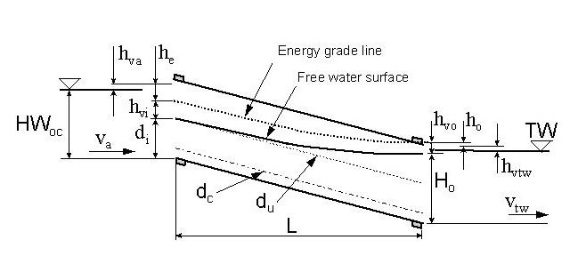
Figure 8-9. Outlet Control Headwater for Culvert with Free Surface
By definition, a free-surface backwater from the outlet end of a culvert may only affect the headwater when subcritical flow conditions exist in the culvert. Subcritical, free-surface flow at the outlet will exist if the culvert is on a mild slope with an outlet depth (H
o
) lower than the outlet soffit or if the culvert is on a steep slope with a tailwater higher than critical depth at the culvert outlet and lower than the outlet soffit.The
is used to determine the water surface profile (and energy losses) though the conduit. The depth, H
o
, is used as the starting depth, d1
. For subcritical flow, the calculations begin at the outlet and proceed in an upstream direction. Use the depth, Ho
, as the starting depth, d1
, in the Direct Step calculations.When using the direct step method, if the inlet end of the conduit is reached without the calculated depth exceeding the barrel depth (D), it verifies that the entire length of the conduit is undergoing free surface flow. Set the calculated depth (d
2
) at the inlet as Hi
and refer to Energy Balance at Inlet to determine the headwater.When using the direct step method, if the calculated depth (d
2
) reaches or exceeds the barrel depth (D), the inside of the inlet is submerged. Refer to Type AB - Free surface at outlet and full flow at inlet for a description. This condition is possible if the theoretical value of uniform depth is higher than the barrel depth.Full Flow in Conduit (Type B)
If full flow is occurring in the conduit, rate of energy losses through the barrel is constant (for steady flow) as seen in Figure 8‑10. The hydraulic grade line is calculated based on outlet depth, H
o
, at the outlet.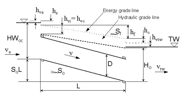
Figure 8-10. Outlet Control, Fully Submerged Flow
Full flow at the outlet occurs when the outlet depth (H
o
) equals or exceeds barrel depth D. Full flow is maintained throughout the conduit if friction slope is steeper than conduit slope, or if friction slope is flatter than conduit slope but conduit is not long enough for the hydraulic grade line to get lower than the top of the barrel.NOTE: Refer to Type BA – Submerged Exit, Free flow at Inlet to determine whether the entire conduit flows full.
Equation 8-11determines the energy loss (friction loss) through the conduit:

Equation 8-11.
where:
- hf= head loss due to friction in the culvert barrel (ft. or m)
- Sf= friction slope (ft. or m) (See Equation 8-13.)
- L= length of culvert containing full flow (ft. or m).
Equation 8-12 is used to compute the depth of the hydraulic grade line at the inside of the inlet end of the conduit. Refer to Energy Balance at Inlet to determine the headwater.
Equation 8-12.
where:
- H= depth of hydraulic grade line at inlet (ft. or m)i
- h= friction head losses (ft. or m) as calculated using Equation 8-11.f
- S= culvert slope (ft./ft. or m/m)o
- L= culvert length (ft. or m)
- Ho= outlet depth (ft. or m).
Equation 8-13 is used to calculate friction slope. If friction slope is flatter than the conduit slope, the hydraulic grade line may drop below the top of the barrel. If this occurs, refer to Type BA - Full Flow at the outlet and free surface flow at the inlet.
Equation 8-13.
where:
S
= friction slope (ft./ft. or m/m)f
- z= 1.486 for English measurements and 1.0 for metric.
Full Flow at Outlet and Free Surface Flow at Inlet (Type BA)
If the friction slope is flatter than the conduit slope, it is possible that full flow may not occur along the entire length of the culvert (see the Table 8-5 on
). The following steps should be followed:
- Determine the length over which full flow occurs (Lf) is using the geometric relationship shown in Equation 8-14 (refer to Table 8-5 on ):
 Equation 8-14.where:
- L= length over which full flow occurs (ft. or m)f
- S= culvert slope (ft./ft. or m/m)o
- S= friction slope (ft./ft. or m/m)f
- H= outlet depth (ft. or m)o
- D= Conduit barrel height (ft. or m).
Use the following table to determine how to proceed considering a conduit length L.Table 8-4: Conduit Length (L) Procedure DeterminationIf…Then proceed to…CommentIf Lf≥ LType B energy loss calculationsEntire length of culvert is fullIf Lf< LStep 2.Outlet is full but free surface flow at inlet - Determine Type BA free surface losses, if applicable. Free surface flow begins at the point of intersection of the hydraulic grade line and the soffit of the culvert barrel as shown in Figure 8‑11. If this condition occurs, determine the depth of flow at the inlet using the Direct Step Method with the starting depth (d1) equal to the barrel rise (D) and starting at the location along the barrel at which free surface flow begins.
- Determine Type BA hydraulic grade line at inlet, if applicable. When the inlet end of the conduit is reached using the direct step method, set the calculated depth at the inlet as Hi and refer to Energy Balance at Inlet to determine the headwater.
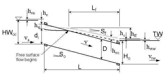 Figure 8-11. Point at Which Free Surface Flow Begins
Free Surface at Outlet and Full Flow at Inlet (Type AB)
When the outlet is not submerged, full flow will begin within the conduit if the culvert is long enough and the flow high enough. Figure 8‑12 illustrates this condition. This condition is possible if the theoretical value of uniform depth is higher than the barrel depth. The following steps should be followed:
- Check Type AB uniform depth. Compare calculated uniform depth and the barrel depth, D. If the theoretical value of uniform depth is equal to or higher than the barrel depth, proceed to Free Surface Losses. Otherwise, refer to .
- Determine Type AB free surface losses, if applicable. Refer to Water Surface Profile Calculations, Free Surface Flow to determine the water surface profile in the conduit. If the computed depth of flow reaches or exceeds the barrel depth before the end of the conduit, note the position along the conduit at which this occurs and proceed to full flow losses below. Otherwise, complete the procedure described under Free Surface Flow.
- Determine Type AB full flow losses, if applicable. Begin full flow calculations at the point along the conduit where the computed water surface intersects the soffit of the barrel as determined above. Determine the energy losses through the remainder of the conduit using Equation 8-11 but substituting Lf, the remaining conduit length, for L.
- Determine Type AB hydraulic grade line at inlet, if applicable. Compute the depth of the hydraulic grade line, Hi, at the inside of the inlet end of the conduit using Equation 8-12. Use the barrel height D as the starting hydraulic grade line depth in place of Ho,and use the remaining length, Lf, in place of L. Refer to Energy Balance at Inlet to determine headwater depth.
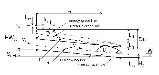 Figure 8-12. Headwater Due to Full Flow at Inlet and Free Surface at Outlet
Energy Balance at Inlet
The outlet control headwater, HW
oc
, is computed by balancing the energy equation, depicted as Equation 8-15. The hydraulic grade at the inside face of the culvert at the entrance will need to be known. See
. The velocity at the entrance (vi
) is used to compute the velocity head at the entrance (hvi
).
Equation 8-15.
where:
- HWoc= headwater depth due to outlet control (ft. or m)
- hva= velocity head of flow approaching the culvert entrance (ft. or m)
- h= velocity head in the entrance (ft. or m) as calculated using Equation 8-9vi
- he= entrance head loss (ft. or m) as calculated using Equation 8-16
- Hi= depth of hydraulic grade line just inside the culvert at inlet (ft. or m).Generally, when using Equation 8-15, the velocity approaching the entrance may be assumed to be negligible so that the headwater and energy grade line are coincident just upstream of the upstream face of the culvert. This is conservative for most department needs. The approach velocity may need to be considered when performing the following tasks:
- determining the impact of a culvert on FEMA designated floodplains
- designing or analyzing a culvert used as a flood attenuation device where the storage volumes are very sensitive to small changes in headwater.
The entrance loss, h
e
, depends on the velocity of flow at the inlet, vi
, and the entrance configuration, which is accommodated using an entrance loss coefficient, Ce
.
Equation 8-16.
where:
- Ce= entrance loss coefficient
- Vi= flow velocity inside culvert inlet(fps or m/s).
NOTE: The pipes of pipe runner SETs have been proven to be within the tolerance of the entrance loss equations. Therefore, the entrance should be evaluated solely for its shape and the effect of the pipes should be ignored.
Values of C
e
are shown on the following table (Entrance Loss Coefficients) based on culvert shape and entrance condition. (AASHTO Highway Drainage Manual Guidelines, 4th Ed, Table 4-1)Concrete Pipe | C e |
|---|---|
Projecting from fill, socket end (groove end) | 0.2 |
Projecting from fill, square cut end | 0.5 |
Headwall or headwall and wingwalls: | - |
| 0.2 |
| 0.5 |
| 0.2 |
Mitered to conform to fill slope | 0.7 |
End section conforming to fill slope | 0.5 |
Beveled edges, 33.7º or 45º bevels | 0.2 |
Side- or slope-tapered inlet | 0.2 |
Corrugated Metal Pipe or Pipe Arch | - |
Projecting from fill (no headwall) | 0.9 |
Headwall or headwall and wingwalls square-edge | 0.5 |
Mitered to conform to fill slope, paved or unpaved slope | 0.7 |
End section conforming to fill slope | 0.5 |
Beveled edges, 33.7º or 45º bevels | 0.2 |
Side- or slope-tapered inlet | 0.2 |
Reinforced Concrete Box | - |
Headwall parallel to embankment (no wingwalls): | - |
| 0.5 |
| 0.2 |
Wingwalls at 30º to 75º to barrel: | - |
| 0.4 |
| 0.2 |
Wingwall at 10º to 25º to barrel: square-edged at crown | 0.5 |
Wingwalls parallel (extension of sides): square-edged at crown | 0.7 |
Side- or slope-tapered inlet | 0.2 |
Slug Flow
When the flow becomes unstable, a phenomenon termed slug flow may occur. In this condition the flow oscillates between inlet control and outlet control due to the following instances:
- Flow is indicated as supercritical, but the tailwater level is relatively high.
- Uniform depth and critical depth are relatively high with respect to the culvert barrel depth.
- Uniform depth and critical depth are within about 5% of each other.
The methods recommended in this chapter accommodate the potential for slug flow to occur by assuming the higher of inlet and outlet control headwater.
Determination of Outlet Velocity
The outlet velocity, v
o
, depends on the culvert discharge (Q) and the cross-sectional area of flow at the outlet (Ao
) as shown in Equation 8-17.
Equation 8-17.
- Assign the variable doas the depth with which to determine the cross-sectional area of flow at the outlet.
- For outlet control, set the depth, do,equal to the higher of critical depth (dc) and tailwater depth (TW) as long as the value is not higher than the barrel rise (D) as shown in Figure 8‑13.
- If the conduit will flow full at the outlet, usually due to a high tailwater or a conduit capacity lower than the discharge, set doto the barrel rise (D) so that the full cross-sectional area of the conduit is used as shown in Figure 8‑14.
Figure 8-13. Cross Sectional Area based on the Higher of Critical Depth and Tailwater
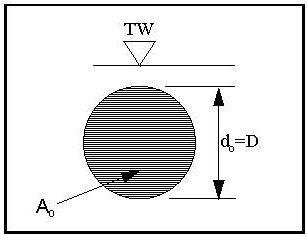
Figure 8-14. Cross Sectional Area Based on Full Flow
Depth Estimation Approaches
For inlet control under steep slope conditions, estimate the depth at the outlet using one of the following approaches:
- Use a step backwater method starting from critical depth (dc) at the inlet and proceed downstream to the outlet: If the tailwater is lower than critical depth at the outlet, calculate the velocity resulting from the computed depth at the outlet. If the tailwater is higher than critical depth, a hydraulic jump within the culvert is possible. The subsection below discusses a means of estimating whether the hydraulic jump occurs within the culvert. If the hydraulic jump does occur within the culvert, determine the outlet velocity based on the outlet depth, do= Ho.
- Assume uniform depth at the outlet. If the culvert is long enough and tailwater is lower than uniform depth, uniform depth will be reached at the outlet of a steep slope culvert: For a short, steep culvert with tailwater lower than uniform depth, the actual depth will be higher than uniform depth but lower than critical depth. This assumption will be conservative; the estimate of velocity will be somewhat higher than the actual velocity. If the tailwater is higher than critical depth, a hydraulic jump is possible and the outlet velocity could be significantly lower than the velocity at uniform depth.
Direct Step Backwater Method
The Direct Step Backwater Method uses the same basic equations as the Standard Step Backwater Method but is simpler to use because no iteration is necessary. In the Direct Step Method, an increment (or decrement) of water depth (δd) is chosen and the distance over which the depth change occurs is computed. The accuracy depends on the size of δd. The method is appropriate for prismatic channel sections such as occur in most conduits. It is useful for estimating supercritical profiles and subcritical profiles.
- Choose a starting point and starting water depth (d1). This starting depth depends on whether the profile is supercritical or subcritical. Generally, for culverts, refer to outlet depth and set d1to the value of H0. Otherwise, you may use the following conditions to establish d1:
- For a mild slope (dc< du) and free surface flow at the outlet, begin at the outlet end. Select the higher of critical depth (dc) and tailwater depth (TW). Supercritical flow may occur in a culvert on a mild slope. However, most often, the flow will be subcritical when mild slopes exist. Check this assumption.
- For a steep slope (dc> du), where the tailwater exceeds critical depth but does not submerge the culvert outlet, begin at the outlet with the tailwater as the starting depth.
- For a steep slope in which tailwater depth is lower than critical depth, begin the water surface profile computations at the culvert entrance starting at critical depth and proceed downstream to the culvert exit. This implies inlet control, in which case the computation may be necessary to determine outlet velocity but not headwater.
- For a submerged outlet in which free surface flow begins along the barrel, use the barrel depth, D, as the starting depth. Begin the backwater computations at the location where the hydraulic grade line is coincident with the soffit of the culvert.
- The following steps assume subcritical flow on a mild slope culvert for a given discharge, Q, through a given culvert of length, L, at a slope, So. Calculate the following at the outlet end of the culvert based on the selected starting depth (d1):
- cross-section area of flow, A
- wetted perimeter, WP
- velocity, v, from Equation 8-17
- velocity head, hv, using Equation 8-9
- specific energy, E, using Equation 8-18
- friction slope, Sf, using Equation 8-13.
- Assign the subscript 1 to the above variables (A1, WP1, etc.).
 Equation 8-18.where:
- E= specific energy (ft. or m)
- d= depth of flow (ft. or m)
- v= average velocity of flow (fps or m/s)
- g= gravitational acceleration = 32.2 ft/ s2or 9.81 m/s2.
- Choose an increment or decrement of flow depth, δ d: if d1> du, use a decrement (negative δ d); otherwise, use an increment. The increment, δ d, should be such that the change in adjacent velocities is not more than 10%.
- Calculate the parameters A, WP, v, E, and Sfat the new depth, d2= d1+ δ d, and assign the subscript 2 to these (e.g., A2, WP2, etc.).
- Determine the change in energy, δ E, using Equation 8-19.
- Calculate the arithmetic mean friction slope using Equation 8-20.
- Using Equation 8-21, determine the distance, δ L, over which the change in depth occurs.
- Consider the new depth and location to be the new starting positions (assign the subscript1to those values currently identified with the subscript2) and repeat steps 3 to 7, summing the incremental lengths, δ L, until the total length, Σ L, equals or just exceeds the length of the culvert. You may use the same increment throughout or modify the increment to achieve the desired resolution. Such modifications are necessary when the last total length computed far exceeds the culvert length and when high friction slopes are encountered. If the computed depth reaches the barrel rise (D) before reaching the culvert inlet, skip step 9 and refer to the to complete the analysis.
- The last depth (d2) established is the depth at the inlet (Hi) and the associated velocity is the inlet, vi. Calculate the headwater using Equation 8-15.
 Equation 8-19.
 Equation 8-20.
 Equation 8-21.
Subcritical Flow and Steep Slope
The procedure for subcritical flow (d > d
c
) but steep slope (dc
> du
) is similar with the following exceptions:- Choose a decrement in depth, δd = negative.
- If the depth, d, reaches critical depth before the inlet of the culvert is reached, the headwater is under inlet control ( ) and a may occur in the culvert barrel (refer to the following subsection for discussion of the hydraulic jump in culverts).
- If the depth at the inlet is higher than critical depth, determine the outlet control head using Equation 8-15 as discussed in the subsection. A hydraulic jump may occur within the culvert.
Supercritical Flow and Steep Slope
The procedure for supercritical flow (d < d
c
) and steep slope is similar with the following exceptions:- Begin computations at critical depth at the culvert entrance and proceed downstream.
- Choose a decrement of depth, δd.
- If the tailwater is higher than critical depth, a hydraulic jump may occur within the culvert (refer to the following subsection for discussion of the hydraulic jump).
Hydraulic Jump in Culverts
Figure 8-15 provides a sample plot of depth and momentum function and an associated specific energy plot. For a given discharge and given energy and momentum, there exist two possible depths, one less than critical depth (supercritical flow) a sequent (or conjugate) depth greater than critical depth (subcritical flow). With a proper configuration, the water flowing at the lower depth in supercritical flow can “jump” abruptly to its sequent depth in subcritical flow. This is called a hydraulic jump. With the abrupt change in flow depth comes a corresponding change in cross-sectional area of flow and a resulting decrease in average velocity.
By comparing the two curves at a supercritical depth and its sequent depth, it is apparent that the hydraulic jump involves a loss of energy. Also, the momentum function defines critical depth as the point at which minimum momentum is established.
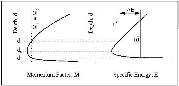
Figure 8-15. Momentum Function and Specific Energy
The balance of forces is represented using a momentum function (Equation 8-22):
Equation 8-22.
where:
- M= momentum function
- Q= discharge (cfs or m3/s)
- g = gravitational constant = 32 ft./sec2
- A= section area of flow (sq. ft. or m2)
= distance from water surface to centroid of flow area (ft. or m).
The term A
represents the first moment of area about the water surface. Assuming no drag forces or frictional forces at the jump, conservation of momentum maintains that the momentum function at the approach depth, M
represents the first moment of area about the water surface. Assuming no drag forces or frictional forces at the jump, conservation of momentum maintains that the momentum function at the approach depth, M
1
, is equal to the momentum function at the sequent depth, Ms
.The potential occurrence of the hydraulic jump within the culvert is determined by comparing the outfall conditions with the sequent depth of the supercritical flow depth in the culvert. The conditions under which the hydraulic jump is likely to occur depend on the slope of the conduit.
Under mild slope conditions (d
c
< du
) with supercritical flow in the upstream part of the culvert, the following two typical conditions could result in a hydraulic jump:- The potential backwater profile in the culvert due to the tailwater is higher than the sequent depth computed at any location in the culvert.
- The supercritical profile reaches critical depth before the culvert outlet.
Under steep slope conditions, the hydraulic jump is likely only when the tailwater is higher than the sequent depth.
Sequent Depth
A direct solution for sequent depth, d
s
is possible for free surface flow in a rectangular conduit on a flat slope using Equation 8-23. If the slope is greater than about 10 percent, a more complex solution is required to account for the weight component of the water. FHWA
provides more detail for such conditions.
Equation 8-23.
where:
- d= sequent depth, ft. or ms
- d= depth of flow (supercritical), ft. or m1
- v= velocity of flow at depth d, ft./s or m/s.1
A direct solution for sequent depth in a circular conduit is not feasible. However, an iterative solution is possible by following these equations:
- Select a trial sequent depth, ds, and apply Equation 8-24 until the calculated discharge is equal to the design discharge. Equation 8-24 is reasonable for slopes up to about 10 percent.
- Calculate the first moments of area for the supercritical depth of flow, d1, and sequent depth, ds, using Equation 8-25.
- This equation uses the angle β shown in Figure 8‑16, which you calculate by using Equation 8-26.
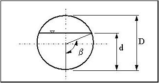 Figure 8-16. Determination of Angle bCAUTION: Some calculators and spreadsheets may give only the principal angle for β in Equation 8-26 (i.e., -π/2 radians ≤ β ≤ π/2 radians).
 - Use Equation 8-27 to calculate the areas of flow for the supercritical depth of flow and sequent depth.
 Equation 8-24.
where:
- Q= discharge, cfs or m3/s
- As= area of flow at sequent depth, sq.ft. or m2
- A= first moment of area about surface at sequent depth, cu.ft. or msds3
- A= first moment of area about surface at supercritical flow depth, cu.ft. or m1d13.
Equation 8-25.
where:
- Ad= first moment of area about water surface, cu.ft. or m3
- D= conduit diameter, ft. or m
- β = angle shown in Figure 8‑16 and calculated using Equation 8-26.
Equation 8-26.
Equation 8-27.
Equation 8-24 applies to other conduit shapes having slopes of about 10 percent or less. The first moment of area about the surface, A
, is dependent on the shape of the conduit and depth of flow. A relationship between flow depth and first moment of area must be acquired or derived.
, is dependent on the shape of the conduit and depth of flow. A relationship between flow depth and first moment of area must be acquired or derived.
Roadway Overtopping
Where water flows both over the roadway and through a culvert (see Figure 8‑17), a flow distribution analysis is required to define the hydraulic characteristics. This is a common occurrence where a discharge of low design AEP (low probability of occurrence) is applied to a facility designed for a lower design frequency.
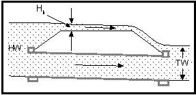
Figure 8-17. Culvert with Overtopping Flow
For example, a complete design involves the application and analysis of a 1% AEP discharge to a hydraulic facility designed for a much smaller flood. In such a case, the headwater may exceed the low elevation of the roadway, causing part of the water to flow over the roadway embankment while the remainder flows through the structure. The headwater components of flow form a common headwater level. An iterative process is used to establish this common headwater.
The following procedure is an iterative approach that is reasonable for hand computations and computer programs:
- Initially assume that all the runoff (analysis discharge) passes through the culvert, and determine the headwater. Use the procedures outlined in the section. If the headwater is lower than the low roadway elevation, no roadway overtopping occurs and the analysis is complete. Otherwise, proceed to step 2.
- Record the analysis discharge as the initial upper flow limit and zero as the initial lower flow limit. Assign 50% of the analysis discharge to the culvert and the remaining 50% to the roadway as the initial apportionment of flow.
- Using the procedures outlined in the section, determine the headwater with the apportioned culvert flow.
- Compute the roadway overflow (discharge) required to subtend the headwater level determined in step 3 using Equation 8-28.
 Equation 8-28.where:
- Q= discharge (cfs or m3/s)
- kt= over-embankment flow adjustment factor (see Figure 8‑18)
- C= discharge coefficient (use 3.0 – English or 1.66 metric for roadway overtopping)
- L= horizontal length of overflow (ft. or m). This length should be perpendicular to the overflow direction. For example, if the roadway curves, the length should be measured along the curve.
- Hh= average depth between headwater and low roadway elevation (ft. or m).
- Base the value Hhon the assumption that the effective approach velocity is negligible. For estimation of maximum headwater, this is a conservative assumption. However, under some conditions, such as the need to provide adequate detention storage, you may need to consider the approach velocity head (v2/2g). That is, replace Hhin Equation 8-28 with Hh+ v2/2g.
- With reference to Figure 8‑19, the flow over the embankment will not be affected by tailwater if the excess (Ht) is lower than critical depth of flow over the road (approximately 0.67 Hh) . For practical purposes, Ht/Hhmay approach 0.8 without any correction coefficient. For Ht/Hhvalues above 0.8 use Figure 8‑18 to determine kt.
- For most cases of flow over highway embankments, the section over which the discharge must flow is parabolic or otherwise irregular (see Figure 8‑20). In such cases, it becomes necessary to divide the section into manageable increments and to calculate individual weir flows for the incremental units, summing them for total flow.
- If the tailwater is sufficiently high, it may affect the flow over the embankment. In fact, at high depth, the flow over the road may become open channel flow, and weir calculations are no longer valid. At extremely high depth of roadway overtopping, it may be reasonable to ignore the culvert opening and compute the water surface elevation based on open channel flow over the road.
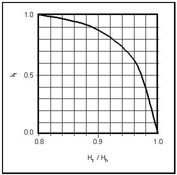 Figure 8-18. Over Embankment Flow Adjustment Factor
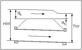 Figure 8-19. Roadway Overtopping with High Tailwater
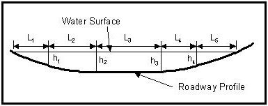 Figure 8-20. Cross Section of Flow over Embankment
 - Add the calculated roadway overflow to the culvert flow. If the calculated total is greater than the analysis discharge, record the current culvert flow apportionment as the current upper flow limit and set the new culvert flow apportionment at a value halfway between the current upper and lower flow limits. If the calculated total is less than the analysis discharge, record the current culvert flow apportionment as the lower flow limit for the culvert and set the new culvert flow apportionment at a value halfway between the current upper and lower flow limits.
- Repeat steps 3 to 5, using the culvert flow apportionment established in step 5, until the difference between the current headwater and the previous headwater is less than a reasonable tolerance. For computer programs, the department recommends a tolerance of about 0.1 in. The current headwater and current assigned culvert flow and calculated roadway overflow can then be considered as the final values.
Performance Curves
For any given culvert, the control (outlet or inlet) might vary with the discharge. Figure 8‑18 shows sample plots of headwater versus discharge for inlet and outlet control. The envelope (shown as the bold line) represents the highest value of inlet and outlet headwater for any discharge in the range. This envelope is termed a performance curve.
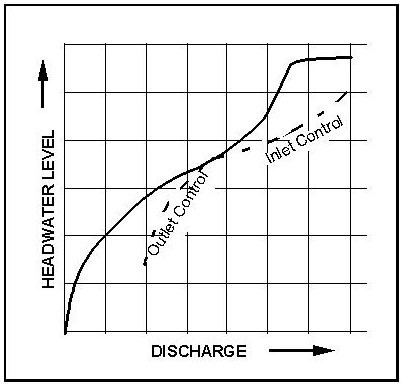
Figure 8-21. Typical Performance Curve
In this example, inlet control prevails at lower discharges and flow transitions to outlet control as the discharge increases. The flatter portion represents the effect of roadway overflow. The performance curve can be generated by calculating the culvert headwater for increasing values of discharge. Such information is particularly useful for performing risk assessments and for hydrograph routing through detention ponds and reservoirs.
Exit Loss Considerations
The traditional assumption in the design of typical highway culverts is continuity of the hydraulic grade line. At the outlet, this implies that when the tailwater is higher than critical depth and subcritical flow exists, the hydraulic grade line immediately inside the barrel is equal to the tailwater level. This is reasonable for most normal culvert designs for TxDOT application. However, by inference there can be no accommodation of exit losses because the energy grade line immediately inside the culvert can only be the hydraulic grade line plus the velocity head, no matter what the velocity is in the outfall.
Occasionally, an explicit exit loss may need to be accommodated. Some examples are as follows:
- conformance with another agency’s procedures
- comparison with computer programs (such as HEC-RAS)
- design of detention pond control structures in which storage volumes are sensitive to small changes in elevation.
If such a need arises, base the starting hydraulic grade level (H
o
) is based on balancing
between the outside and inside of the culvert face at the outlet. A common expression for exit loss appears in Equation 8-30. This assumes that the tailwater velocity (vTW
) is lower than the culvert outlet velocity (vo
) and the tailwater is open to the atmosphere. If the above approach is used, it is most likely that the outlet depth (Ho
) will be lower than the tailwater. This conforms to basic one-dimensional hydrostatic principles.
Equation 8-29.
where:
- Ho= outlet depth - depth from the culvert flow line to the hydraulic grade line inside the culvert at the outlet (ft. or m)
- vo= culvert outlet velocity (ft./s or m/s)
- v= velocity in outfall (tailwater velocity) (ft./s or m/s)TW
- ho= exit loss (ft. or m).
Equation 8-30.
where:
- K= loss coefficient which typically varies from 0.5 to 1.