13.5 Calibration
13.5.1 Overview
To validate a model’s accuracy, the model is recommended to report results that are not only representative of the model but that also match results to real-world conditions. Previous model debugging indicates that reported results are representative of what is occurring in the network which instills confidence in model results. Before a model is deemed reliable, calibrate it to certify that the results match the real-world conditions it was based on. The goal of calibration is to find the set of parameter values that best mimics observed measures. The following section provides guidance on calibration thresholds and methodology. The majority of the discussion in this section is based on the FHWA 2019 Guidelines.
Calibration is the adjustment of various model parameters to improve the accuracy of the model’s results. Parameters are modified to create congestion patterns that are accurate to observed data, such as how congestion forms and dissipates over time under specific conditions. Default parameters are not considered calibrated.
Per the FHWA 2019 Guidelines, calibration is applied using data from a single representative day. Model results are analyzed with a single Random Seed run. Note that this is different from the
FHWA Traffic Analysis Toolbox, Volume III
(2004) Guidelines, where model results for calibrated models were analyzed from an average of multiple Random Seed runs. It is still recommended that a model be ran with multiple Random Seeds to check for any errors in coding and errors that might cause gridlock conditions. A few common reasons for gridlock include vehicles, pedestrians, bicycles stuck in an unsolvable conflict, or a missing detector at an actuated, signalized intersection. The model is typically debugged further before continuing the calibration process.FHWA 2004 Guidelines may be followed for traffic analysis for TxDOT projects that do not involve FHWA approval. Average day traffic analysis may be performed for these projects. Follow FHWA 2019 Guidelines for projects that involve IAJRs or FHWA approval. The 2019 guidelines require considerably more data than the 2004 guidelines. If sufficient data is not available or practical to collect, then the use of the 2004 guidelines may be requested as an exception for projects that require FHWA approval.
During calibration, solving one issue often highlights new issues elsewhere. It is crucial to strategize calibration by splitting up the process into logical, sequential steps. A good strategy is to:
- Divide model parameters into two categories; and
- Parameters adjusted during calibration
- Parameters that are to not be adjusted
- Divide the adjustable parameters into global and local parameters
- Global parameters are those that affect the entire network (e.g., specific attributes of the representative day covering the entire network)
- Local parameters are those that affect the parts of the network (e.g., parameter that affects a particular link, movement, speed decision, etc.)
Calibrating a model using DTA is similar to calibration of microscopic traffic simulation models. The basic steps in calibrating a DTA model (as defined in the FHWA
Traffic Analysis Toolbox XIV: Guidebook on the Utilization of Dynamic Traffic Assignment in Modeling
) is as follows:- Establish calibration objectives and review the project objective to confirm that the calibration task directly supports the project objective.
- Identify the performance measures and critical locations against which the models will be calibrated.
- Determine the statistical methodology to be used to compare modeled results to the field data.
- Determine the strategy for model calibration and identify parameters within the DTA models that are the focus of adjustments.
- Assemble field data previously collected for comparison to model outputs.
- Conduct model calibration runs following the strategy and conduct statistical checks. When statistical analysis falls within the acceptable ranges, the model is calibrated.
- Validation: Test or compare the calibrated model with a data set not used for calibration. If the model replicates the different data set, the calibration parameters and model are validated.
13.5.2 Acceptability Criteria
Effective calibration demands several performance measures for calibration. This section summarizes the
FHWA Traffic Analysis Toolbox, Volume III (2004)
and FHWA Traffic Analysis Toolbox, Volume III (2019)
Guidelines for calibration. For all FHWA related projects, it is necessary to use the FHWA 2019 Guidelines. For non-FHWA projects, calibration criteria is typically determined during project scoping and based on discussions with the TxDOT project manager. If a non-FHWA project is in an urban area and the data is available, it is recommended to use the FHWA 2019 Guidelines.13.5.2.1 FHWA Traffic Analysis Toolbox, Volume III (2004) Requirements
The previous FHWA 2004 Guidelines provided guidance on calibrating travel times and throughputs. To consider a model calibrated, at least two metrics are calibrated. The calibration criteria only apply to the peak hour.
13.5.2.2 Travel Time
Travel time calibration criteria are separated into two types of roadway facilities: uninterrupted flow and interrupted flow. To calibrate a model, the allowable travel time variation is measured using the equations shown in
Facility Type | Equation |
|---|---|
Free-Flowing | 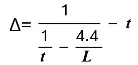 |
Interrupted Flow | 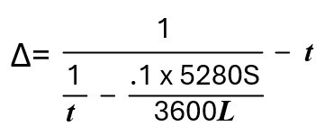 |
∆ = Allowable Travel Time Variation (+/- seconds)
t = Real-World Travel Time (seconds)
L = Length (ft)
S = Free Flow Speed (FFS) in mph; Posted Speed can be used for FFS if unknown
13.5.2.3 Throughput
To measure and compare field data and simulation throughputs, this guidance uses the Geoffrey E. Havers (GEH) formula. The GEH statistic is typically calculated for mainline segments and ramps. It is recommended that calibration of the model using the GEH formula is calculated to a value of 3 or lower:
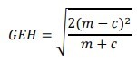
where,
m = output traffic throughput volumes from the simulation model (veh/h/ln)
c = traffic throughput volumes based on field data (veh/h/ln)
Additional criteria for GEH statistics are shown in and .
GEH Statistics | Guidance |
|---|---|
< 3.0 | Acceptable Fit |
3.0 to 5.0 | Acceptable for Local Roadway Facilities |
> 5.0 | Unacceptable |
Criteria | Acceptable Targets |
|---|---|
GEH < 3.0 | All State facility segments within the calibration area |
GEH < 3.0 | All points of entry and exit locations within the calibration area |
GEH < 3.0 | All entrance and exit ramps within the calibration area |
GEH < 5.0 | At least 85% of applicable local roadway segments |
Sum of all segment flows within the calibration area | Within 5% |
13.5.2.4 FHWA Traffic Analysis Toolbox, Volume III (2019) Requirements
The FHWA 2019 Guidelines has four separate acceptability criteria. These calibration criteria are recommended for projects that involve FHWA review and approval. Each calibration criterion can be applied to all performance metrics that are being used for calibration purposes such as travel time routes, throughputs, etc.
The first two are related to sigma bands and the last two are related to accuracy. Sigma bands contain the number of outliers and inliers in the simulated results. Using graphical representation, the simulated data typically fits between the upper and lower limits of the sigma band criterion.
- Criterion I is Control for Time-Variant “Outliers”. The purpose of this criterion is to control for maximum number of outliers associated with the simulation results. To fulfill this criterion, the 2- sigma band criterion, 95 percent of all simulated data points are contained within the 2-sigma band thresholds. Note that if fewer than 20 time-intervals are used for the analysis, then a maximum of one value may fall outside of the time-variant envelope.
- Criterion II is Control for Time-Variant “Inliers”. The purpose of this criterion is to constrain the simulated results to fall closely in line with the representative day. To satisfy this criterion, the 1-sigma band criterion, 66 percent of all simulated data points are contained within the 1-sigma thresholds, and simulated results for 2 non-adjacent critical time intervals are within the time-variant envelope. below shows the time-variant envelopes for the representative day travel times for Criterion I (2 sigma band) and Criterion II (1 sigma band).
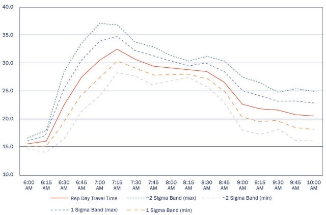
Figure 13-6: Sample Chart Plot of Variation Envelope for Travel Times from FHWA
- Calibration Criterion III is the Bounded Dynamic Absolute Error (BDAE) and verifies that the data accurately captures the data from the representative day. The BDAE is calculated before comparing the simulated results against it. The following equations are used to calibrate for Criteria III and Criteria IV:
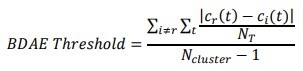
where,
Cr(𝑡) = Observed value of representative day (r) during time interval t
Ci(𝑡) = Observed value of non-representative day (i) within the cluster during time interval t
Csi(𝑡𝑡) = Simulated performance measure during time interval t
N
= Number of time intervals T
N
= Number of days in the cluster representing this travel conditioncluster
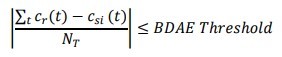
Criterion III checks the simulated data with the field data to determine whether it is an overestimate or underestimate for the calibration metrics. The following equation is used to calibrate for Criterion III:
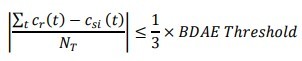
- Calibration Criterion IV, Bounded Dynamic Systematic Error, checks for the simulated data against the field data to determine whether it is an overestimate or underestimate for the calibration metrics. The following equation is used to calibrate for Criteria IV:
A detailed
example
of the calibration criteria calculations is provided in Appendix N, Section 3 – Calibration Criteria Calculations Example
. Comparison Summary between FHWA 2004 and 2019 Guidelines:
There are several differences between the FHWA 2004 and 2019 calibration guidelines. Although, calibration is still performed on similar performance measures such as travel time, throughput, queues, etc., the approach is very different when comparing the two guidance documents. Instead of each performance measure having different sets of calibration acceptance targets, all performance measures are analyzed using the same four criteria in the FHWA 2019 Guidelines. The FHWA 2019 Guidelines also has a heavy emphasis on collecting a larger amount of data for calibration. shows a comparison between the two guidance documents.
Calibration Parameter | 2004 | 2019 |
|---|---|---|
Calibration for an average day | X | |
Calibration for a single representative day | X | |
Hourly flows (individual links and sum of all links) | X | |
Travel times (within 15%, or 1 min, if higher) | X | |
GEH statistics (individual link flows and sum of all link flows) | X | |
Visual audits (queues/bottle necks) | X | X |
Bottleneck throughputs | X | X |
Calibration for saturation flow rate | X | X |
Criterion I – Control for time-variant outliers | X | |
Criterion II – Control for time-variant “inliers” | X | |
Criterion III – Bounded Dynamic Absolute Error (BDAE) | X | |
Criterion IV – Bounded Dynamic Systematic Error | X |
13.5.3 Calibration Parameters and Best Practices
Calibration demands several iterations of adjustments to calibrate to real-world conditions. There are several model parameters that are typically attuned to the collected field data. The calibration of a model relies on the data collected. presents various calibration measures and potential data sources
Calibration Measure | Facility | Potential Data Sources | Potential Output Files |
|---|---|---|---|
Volume/Throughput | Freeway/Ramps | Tube or video counts | Link evaluation, Data collection points |
Arterials/Intersections | Tube, video, or manual counts | Link/node evaluation, Data collection points | |
Travel Times | Freeways/Arterials | Field Travel Time Runs or Probe Data | Travel time segments |
Speed/Congestion | Freeways/Arterials | Spot-Speed Data Collection or Probe Data | Data collection points, Travel time segments |
Bottleneck Locations | Freeways/Arterials | Field photographs/videos/notes or recent peak period aerial imagery (if available) | Visual inspection of model |
Microsimulation calibration best practices are summarized below:
- Select key performance measures for each project. Calibrate selectively for those performance measures.
- Use reliable observed data for the performance measures used for calibration.
- Calibrate based on study area dynamics (bottleneck throughput or duration) and time-variant (travel time, speed) performance measures.
- Use a representative day for calibration rather than an average day that combines multiple days.
The following sections outline possible parameters for calibrating Vissim, CORSIM, and Trafficware’s SimTraffic models.
13.5.3.1 Vissim Calibration
Several parameters can be adjusted in Vissim to fully calibrate a model. The most impactful and common parameters are outlined below:
13.5.3.1.1 Lane Change Parameters
Two common parameters related to lane change behavior are the LCD and the Emergency Stop Distance (ESD). LCD is the point at which a vehicle attempts to change lanes prior to a decision point (e.g., a turning movement). The default LCD setting of 656.2 feet may cause vehicles to switch lanes too late. ESD is defined as the location where vehicles decide to stop and wait for a lane change. These two parameters have great effects on upstream traffic, so their calibration greatly improves a model’s accuracy. Additionally, the following parameters are calibrated in Vissim; reference the Vissim user guide for more guidance:
- Advanced Merge;
- Safety Distance Reduction Factor;
- Cooperative Lane Change; and
- Maximum Deceleration of Own Vehicle (MDOV)
13.5.3.1.2 Speed Distributions
The speed distribution curve in Vissim is set to represent the speed distributions from the collected field data. The posted speed limits are defined as 85 percent of the desired speed distribution in Vissim. Maximum speed distributions is recommended to be set no greater than 10 mph above the speed limit and no less than 5 mph below the speed limit. When calibrating speed distributions, it is possible to increase the percentage of vehicles traveling at the speed or the maximum speed limit cap based on field data.
13.5.3.1.3 Driving Behavior
The interaction between vehicles is modeled using the Wiedemann 1974 and 1999 carfollowing models. Such models are assigned for different driving behavior containers. The Wiedemann 1974 is used for ‘Urban (motorized)’ link types that represent urban arterial roads and streets. The Wiedemann 1999 is primarily used for ‘Freeway (free lane selection)’ link types to model freeway operations. With updated parameters, Wiedemann 1999 is often used for ‘Cycle-Track (free overtaking)’ links to model bicycle lanes. The link type ‘Footpath (no interaction)’ does not monitor the interaction between users of this link type. As such, it can be used for pedestrian movements and walkways and crosswalks. shows all the carfollowing parameters in a Vissim model that can be changed. However, it is recommended to only modify CC0, CC1, and CC2 when adjusting the car-following parameters. Car following and lane changing parameters are shown in .
Parameter | Description |
|---|---|
CC0 | Standstill distance. The distance between two vehicles when they are not moving |
CC1 | Following distance. A time distribution of the speed-dependent portion of safety distance. |
CC2 | Longitudinal oscillation. Defines the distance in which a driver will intentionally move closer to the car it is following. |
CC3 | Perception threshold for following. Defines when the beginning of the deceleration process occurs. |
CC4 | Negative speed difference. Low values result in more sensitive reactions when following vehicles. |
CC5 | Positive speed difference. Low values result in more sensitive reactions when following vehicles. |
CC6 | Influence speed on oscillation. Defines how car-following distance impacts the acceleration of vehicles. |
CC7 | Oscillation acceleration value. Minimum value used when a driver is following another vehicle. |
CC8 | Acceleration value when starting from a standstill. |
CC9 | Acceleration value at 80 km/h |
Diffusion Time | This is the maximum amount of time that a vehicle can wait at an ESD before the vehicle is removed from the network |
Min. Clearance | The minimum distance between two vehicles after a lane change occurs |
Safety distance reduction factor | The safety distance of a following vehicle after a lane change, the safety distance of the vehicle making the lane change, and the distance to the preceding, slower lane change. |
Maximum deceleration for cooperative braking | Defines how much a trailing vehicle will brake to allow an adjacent vehicle to change into its lane. |
Use implicit stochastics | When this option is checked, safety distance, desire acceleration, desired deceleration, minimum lateral distance is stochastic to reflect variations in human perception. When this option is not checked, the characteristics listed above are non-variable. |
13.5.4 CORSIM Calibrating Capacity at Bottlenecks
Calibrating a CORSIM model begins with a calibration of the capacity at key bottlenecks. Replicate the location and severity of bottlenecks, if present. This can be accomplished by evaluating a few key locations in the model and adjusting model parameters in a repeatable process that adjusts throughput volume downstream of the bottleneck until throughputs and queues are similar to local conditions.
When calibrating capacity on a freeway, there are several model parameters that can be adjusted. The parameters and their definitions are listed here:
- Car-following sensitivity factor– A global parameter that represents the primary factor used to calculate headway between a lead-follow pair. The higher the value the more space between vehicles and therefore a lower freeway capacity.
- Car-following sensitivity multiplier– This parameter is adjusted for individual segments. A higher value represents more space between vehicles and therefore a lower freeway capacity.
- Lag acceleration and deceleration time– A global parameter that represents the reaction time necessary for drivers to accelerate or decelerate. A higher value represents a slower reaction time and therefore a lower freeway capacity.
- Pitt car-following constant– A global parameter that represents the minimum amount of space between the rear of the lead vehicle and the front of the follow vehicle. A higher value represents more space between the vehicles and therefore a lower freeway capacity.
When calibrating capacity on surface streets there are several model parameters that can be adjusted. The parameters and their definitions are listed here:
- Mean discharge headway– This parameter is adjusted for individual segments and represents the mean headway between the rear of the lead vehicle and the front of the follow vehicle in a standing queue. A higher value represents a longer headway and therefore a lower capacity.
- Mean startup delay– This parameter is adjusted for individual segments and represents the mean startup lost time for the first vehicle in a standing queue. A higher value represents a greater startup delay and therefore a lower capacity.
- Acceptable gap in oncoming traffic (left turns and right turns)– These are global parameters that represents the minimum acceptable gap in seconds for left turns and right turns. A higher value represents a higher minimum acceptable gap and therefore lower capacity.
- Cross-street acceptable gap distribution (near-side and far-side)– These are global parameters that represent the minimum acceptable gap in seconds at stop signs. A higher value represents a higher minimum acceptable gap and therefore lower capacity.
13.5.5 Calibrating Traffic Volumes
Calibrating the traffic volumes in the model is the second step in calibration and is typically included for all microsimulation models.
This step is completed by comparing the turning movement volumes and link volumes in the model to local conditions. Traffic volumes typically fall within established calibration targets. Traffic volumes are typically calibrated at all locations within the model. If this is not possible for some large networks, calibration of several key locations is acceptable.
When calibrating traffic volumes on a surface street with parallel streets or a network of streets, analysts can use conditional turn movements to define turn percentages. Additionally, a full OD table can be manually coded to minimize differences in modeled volumes.
The FHWA microsimulation guidelines do not demand traffic volume calibration.
13.5.6 Calibrating System Performance
The third calibration step is to calibrate traffic performance in the model to local conditions. Speed, density, travel time, and queue lengths are often used in comparison. It is recommended that system performance is modeled to meet established calibration targets. Methods for calibrating system performance on a freeway are shown here:
Criteria:
- Car-following sensitivity factor, carfollowing sensitivity multiplier, lag acceleration and deceleration time, and Pitt car following constant– these factors are described in detail under the “Calibrating Capacity at Bottlenecks” section and are adjusted to calibrate system performance.
- Time to complete lane change–A global parameter that represents the time a vehicle takes to change lanes. A higher value means the lane change takes longer, but this generally leads to a smoother system performance.
Methods for calibrating system performance on arterials are shown here:
- Mean discharge headway, mean startup delay, acceptable gap in oncoming traffic (left turns and right turns), and cross-street acceptable gap distribution (near-side and far-side)– these factors are described in detail under the “Calibrating Capacity at Bottlenecks” section and are adjusted to calibrate system performance.
- Spillback probabilities– A global parameter that impacts the probability that a vehicle enters an intersection with downstream queues, blocking the intersection.
- Time to react to sudden deceleration of lead vehicle– A global parameter that represents the time it takes for vehicle to begin decelerating after the lead vehicle suddenly decelerates. A higher value represents declined system performance.
Additional information on CORSIM calibration is provided in FHWA Traffic Analysis Toolbox, Volume IV: Guidelines for Applying CORSIM Microsimulation Modeling Software, available here:
Appendix N, Section 4 – External References (Reference 2)
.13.5.7 SimTraffic
Calibration is completed to match field measurements via adhering to established calibration criteria. Calibration in a SimTraffic model includes calibrating travel times, travel volumes, lane alignment, positioning, and crucial distances.