6.1 Safety Analysis Methods

6.1.1 Overall

Chapter 6
provides a detailed overview into the safety analysis methodologies and the tools used to implement safety analysis. Chapter 6
also covers the application of safety analysis methodologies and tools, guidance on safety analysis documentation, and safety analysis applications. An overview of various safety analysis methods is provided in this section. These methods are broken down into existing and future conditions analysis. Figure 6-1

highlights the safety analysis methods covered in this section of the manual.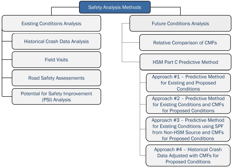

Figure 6-1: Safety Analysis Method

6.1.2 Safety Analysis Study Area

The safety analysis study area includes all roadway elements (segments, intersections, and interchanges) in the area impacted by the proposed project. The traffic analysis study area is a starting point, but the safety analysis area also depends on additional safety impacts of the proposed project. The safety analysis study area limits will be the same for all alternatives for consistency and comparability of the analysis results. Intersections typically include 300 feet on each approach but can be adjusted for intersections where longer queue lengths affect approaches.

6.1.3 Existing Conditions Analysis

The purpose of safety analysis for existing conditions is to identify safety issues that exist and provide the information needed to mitigate those issues. Existing conditions safety analysis methods include the following:

Historical crash data analysis;

Field visits;

Road Safety Assessments (RSAs); and

Potential for Safety Improvements (PSI)

6.1.3.1 Historical Crash Data Analysis

The purpose of a historical crash data analysis is to identify safety issues through the review of crash trends, patterns, and rates. For projects that need FHWA approval, request CRIS data through TxDOT's Traffic Safety Division (TRF) or the Design Division. For other project types, crash data can be obtained through the CRIS website. CRIS allows users to run queries on historical crash data, based on a variety of selection criteria. The CRIS query builder can be used to create a new query, load a saved query, or browse queries authored by TxDOT.

It is recommended that the most recent and complete five calendar years (January 1 through December 31) of crash data be used to conduct a standard historical crash data analysis. It is possible to use less than five years of crash data in the analysis if study area conditions experienced significant changes, resulting in the historical crash data no longer being relevant to the current conditions. For example, a traffic signal installed at an intersection five years ago would result in only four complete calendar years of crash data (beginning after the installation of the traffic signal). In this situation, only use four years of historical crash data for analysis. A minimum of three years of crash data is necessary to perform a historical crash data analysis. If a shorter study period is necessary, pre-approval by the TxDOT Project Manager who will be approving the completed analysis is recommended. The following are situations when a shorter study period may be acceptable:

Recent construction project in the study area;

Before and after study with less than five years of after data; and

Significant land use changes resulting in a significant change in traffic volumes and crash patterns

More than five years of crash data can be used in analysis in certain circumstances. This would be applicable when very little or no historical crash data is available for a study area of interest or when the analysis is focused on a particular subset of crash data that occurs less frequently. For example, using more than five years historical crash data may be applicable when performing historical crash analysis in rural areas with sparce crashes, performing a detailed pedestrian and bicycle crash analysis, or preparing a commercial vehicle crash analysis. When a situation warrants the use of more than five years of crash data, eight years of historical crash data is recommended to be used in the analysis. When a longer study period is necessary, it is to be accepted by the TxDOT Project Manager who will be approving the completed analysis. Table 6-1

shows the recommended years of data recommended for safety analysis on various project types.

Table 6-1: Typical Data Recommendations for Various Project Types
Project Characteristics	Years of Data
Recent construction in the crash area Significant land use changes resulting in change in traffic volumes Performing a before and after study	Review a minimum of 3 years of crash data
Typical historical crash data analysis	Review 5 years of crash data
Analysis of a rural area with few crashes Detailed bicycle and pedestrian analysis Commercial vehicle crash analysis	Review 8 years of crash data

When analyzing historical crash data to determine trends, patterns, and rates, many characteristics should be evaluated and the results can be displayed using a variety of methods. These methods result in the creation of crash summary tables, figures, charts, or maps. The following is a list of minimum characteristics to be included in a historical crash data analysis:

Highway;

Year;

Road part;

Crash location;

Crash severity;

Manner of collision;

Crash rate (include comparison to statewide average for similar facility types);

Segment versus intersection-related;

Pedestrian and bicycle-related; and

Contributing factors

Additional analysis results or characteristics that could be evaluated include, but are not limited to the following:

Weather condition; Traffic and Safety Analysis Procedures Manual | 2024 6-4

Lighting condition;

Road surface condition;

First harmful event;

Vehicle type;

Collision diagrams;

Crash density/heat maps;

Driver age;

Time of day;

Day of week;

Time of year;

Work zone;

Alcohol or drugs;

Speed;

Animal-related; and

Distracted driving

There are methods that can be used to analyze historical crash data and determine crash patterns and trends. Historical crash data analysis includes calculation of crash rates and the comparison of those crash rates to statewide averages for similar facility types. A link to the statewide traffic crash rates is in Appendix G, Section 5 – External References (Reference 11)
. Crash rates are intended to normalize the number of crashes relative to traffic or exposure. When a location or study area is determined to have a crash rate significantly higher than the statewide average (more than five crashes per million entering vehicles for intersections or 5 crashes per 100 million vehicle miles of travel for segments), further analysis may be needed. Crash rates are determined for roadway segments or intersections and can be calculated for total crashes, fatal crashes, injury crashes, and/or fatal and injury crashes.

The equation for determining a crash rate for a roadway segment is:

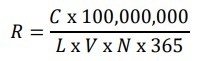
R = Crash rate for the road segment expressed as crashes per 100 million vehicle miles of travel (MVMT)

C= Total number of crashes in the study period

V= Daily traffic volume

L = Length of roadway segment in miles

N = Years of data The equation for determining an intersection crash rate is:

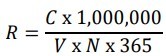
R = Crash rate for the intersection expressed as crashes per 1 million entering vehicles (MEV)

C= Total number of intersection crashes in the study period

V= Traffic volumes entering the intersection daily

N = Years of data

Roadway segment crash rates are calculated per 100 MVMT

Intersection crash rates are typically calculated per MEV. Both MVMT and MEV are traffic exposure variables. For example, if a 6-5 2024 | Traffic and Safety Analysis Procedures Manual two-mile long corridor segment has an AADT or ADT of 20,000 vehicles per day and 50 crashes from 2016 through 2020, the segment crash rate is calculated as follows:

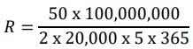
R = 68.5 Crashes per 100 MVMT

Table 6-2

presents an example
of a comparison of crash rates by year for road type and highway system. Crash rates higher than the statewide average indicate the need to further analyze crashes to develop countermeasures and recommend safety improvements. An additional table provided in Appendix G, Section 4 – Example Crash Data Summary
shows crash comparisons by collision type and crash severity. This table is recommended to be used to check whether any aspect of the crash data stands out (e.g., overrepresented crash types or severity, crash rates greater than the statewide average, or patterns of fatalities and suspected serious injuries). Further analysis may be necessary if crash severities are higher than expected, the manner of collisions are different than expected, or if there are issues in unexpected locations. Further analysis can include viewing CR-3 and evaluating crash diagrams.

Table 6-2: Example Crash Rate Comparison
Corridor	Crash Year	Length of Section (mile)	Total Crashes	ADT	Crash Rate	Statewide Average by Road Type (4 or more lanes, undivided)	Statewide Average by Highway System (State Highway)
Main Street	2016	3.0	19	11,934	145.40	104.31	92.43
	2017	3.0	13	12,404	95.71	101.36	90.95
	2018	3.0	17	12,943	119.95	98.43	91.63
	2019	3.0	13	13,755	86.31	95.90	89.17
	2020	3.0	18	14,521	113.20	87.76	79.92

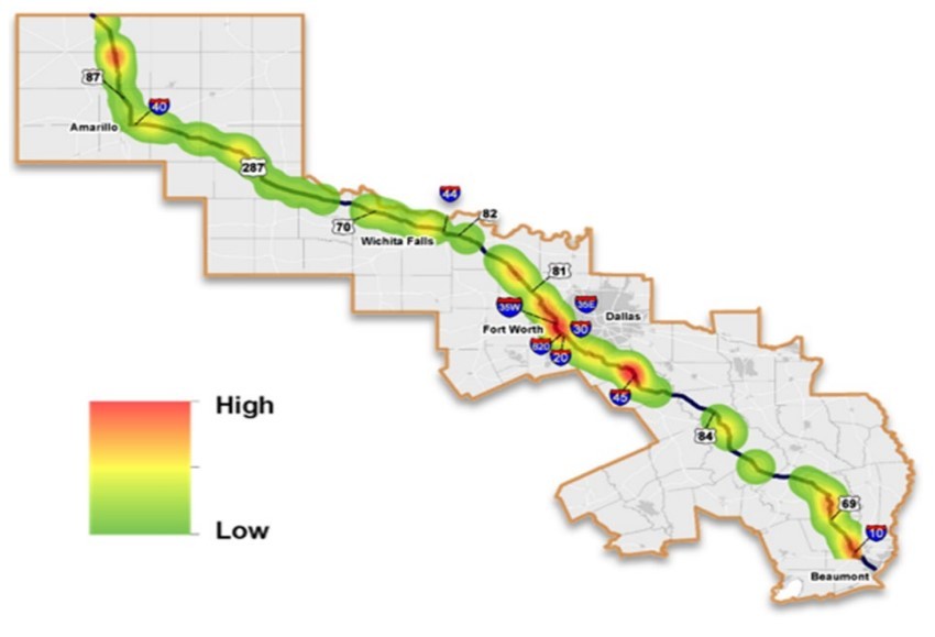
Figure 6-2: Crash Heat Map

Figure 6-2

presents a color-coded crash heat map showing crash concentrated locations (i.e., areas where the density of crashes is high), where green represents a low crash density and red represents a high crash density. These maps are typically created using crash data and a GIS mapping software. They can be helpful in visualizing locations with a high occurrence of crashes. The CRIS query tool also provides an option to view crashes as clusters to visualize crash concentrations. The cluster view combines crashes by area and shows an overall number of crashes.

6.1.3.2 Countermeasures

Proven countermeasures are a collection of strategies that are effective at reducing roadway fatalities and serious injuries. Countermeasures have been developed by FHWA and TxDOT and are shown in Appendix G, Section 5 – External References (Reference 12) and Appendix G, Section 5 – External References (Reference 15)
. These countermeasures are designed to reduce preventable crashes that share specific characteristics. The TxDOT countermeasures consider crashes with the following characteristics:

Part of the roadway the crash occurred on;

First harmful event;

Vehicle movements and manner of collision; and

Type of object struck

Countermeasures are typically used to select strategies to reduce crashes on roadways.

6.1.3.3 Field Visits

A key aspect of performing an existing conditions analysis are field visits. Field visits are used to confirm the existing roadway and traffic operation conditions and can also be used to review the results from the historical crash data analysis. It is recommended that the particular focus of these field visits is to capture information that typically cannot be obtained through the review of historical crash data and predictive analysis. This additional information related to safety can include driver behavior, speed issues, lane utilization, potential conflict issues, and the current conditions of the facility. For example, field visits may be conducted to understand the interaction between vehicles and pedestrians/bicyclists to identify potential safety issues related to these vulnerable user groups. Field visits are usually performed at times specific to the project and may include peak period, off-peak, dusk/dawn, and nighttime visits.

Field visits are recommended to provide additional insight in terms of the local conditions and potential safety issues that could otherwise be missed when only reviewing historical crash data or looking at aerial imagery. The review of aerial imagery or streetlevel photo logs is intended to supplement field visits and are not to be used as a replacement.

6.1.3.4 Road Safety Assessments (RSAs)

One method of supplementing field visits is to follow the formal RSA process as defined in the FHWA Road Safety Audit Guidelines Report (Publication No. FHWA-SA-06-06). The typical RSA includes the following eight steps:

Step 1 – Identify project or road to be audited.

Step 2 – Select an interdisciplinary RSA team that is independent from the project team.

Step 3 – Conduct a pre-assessment meeting to review project information.

Step 4 – Perform field observations under various conditions.

Step 5 – Conduct assessment analysis and prepare report of findings.

Step 6 – Present assessment findings to the project owner.

Step 7 – Project owner prepares formal response.

Step 8 – Incorporate findings into the project, when appropriate.

RSAs can be performed for both existing conditions and proposed design. Generally, projects with the following characteristics benefit from an RSA:

Projects (intersection or road segment) with a low record of safety performance; Traffic and Safety Analysis Procedures Manual | 2024 6-8

Projects with safety issues from stakeholders;

Projects identified during network screening as having lower than expected safety performance; and

Projects using context-sensitive design principles

Additional information about the RSA process is available on the FHWA RSA website, which can be found in Appendix G, Section 5 – External References (Reference 2)
.

6.1.3.5 PSI Analysis

PSI analysis is conducted using the HSM predictive method. The purpose of PSI analysis is to evaluate the existing conditions of the area of interest to determine the potential to reduce crashes at that location. PSI analysis uses the observed crash data at a site to apply the EB method and determine the expected average crash frequency. The difference between the expected average crash frequency and the predicted average crash frequency is the potential reduction in crashes at that site when compared to similar facility types. If the PSI is a positive value (expected crashes are more than predicted crashes) then the site experiences more crashes than would be expected and has the potential to improve safety at that location. Figure 6-3

provides a visual representation of the relationship between observed, predicted, and expected crashes when performing PSI analysis.

The following are the basic analysis steps for performing PSI analysis:

Determine study area;

Determine crash analysis years;

Obtain historical crash data for study area and analysis years;

Calculate predicted average crash frequency using the HSM predictive method for the study area site(s);

Calculate expected average crash frequency by applying the EB method within the HSM predictive method for the study area site(s);

Determine the difference between the expected and predicted crash frequency; and

Document analysis methodology, assumptions, and analysis results

Figure 6-4

contains an example
of one approach for graphically documenting the PSI analysis results.

6.1.4 Future Conditions Analysis

The purpose of safety analysis for future conditions is to consider safety implications of design decisions in the project development process. Future conditions analysis is conducted in a variety of different forms and analysis methods. Future conditions safety analysis methods may include:

Relative Comparison of CMFs for future conditions analysis; and

HSM Part C Predictive Method for future conditions analysis (various approaches)

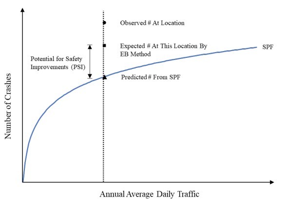
Figure 6-3: Relationship of Observed, Predicted, and Expected Crashes within PSI Analysis

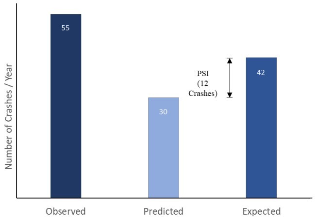
Figure 6-4: Potential for Safety Improvement Example

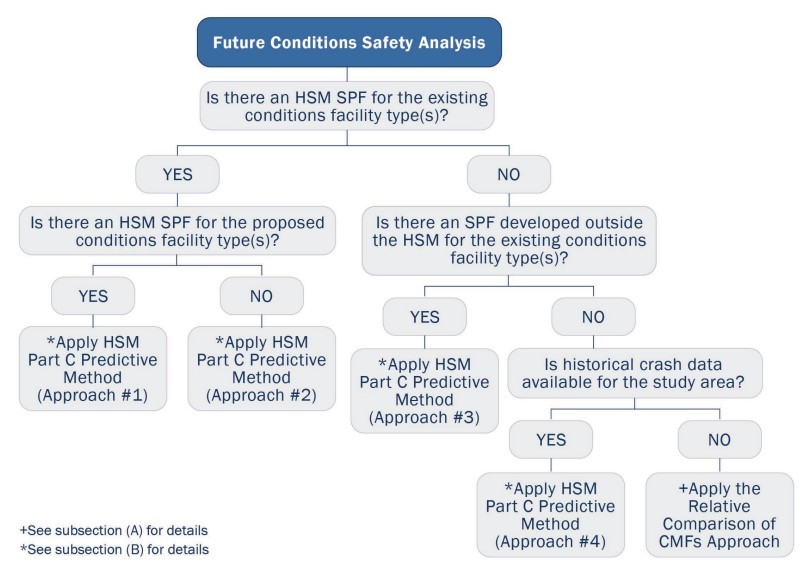
Figure 6-5: Future Conditions Analysis Decision Tree

The decision tree flowchart in Figure 6-5

can be used to determine which of the future conditions safety analysis approaches is best suited for the project. Additional details about the various approaches are provided in the subsequent subsections.

6.1.4.1 Relative Comparison of CMFs

The relative comparison of CMFs method is used to compare the potential safety impacts of alternatives by comparing the CMF values for each of the proposed alternatives or countermeasures. Comparing CMFs involves verifying that the comparisons are of identical crash types and other details. This method is typically used when historical crash data is not available. This method is the simplest method to apply and involves careful selection of CMFs. The relative comparison of CMFs method is most suitable for the initial screening of viable countermeasures before performing a more detailed analysis.

The basic analysis steps when performing a relative comparison of CMFs analysis are as follows:

Determine the safety study area;

Identify the existing conditions and proposed countermeasure(s) or alternative(s);

Determine and document the appropriate CMF(s) for each countermeasure or alternative; and

Use the results to determine next steps for additional analysis, if needed

Table 6-3

provides an example
of how the relative comparison of CMFs analysis method could be applied. This example considers various alternatives for pedestrian facility modifications using CMFs located on the CMF Clearinghouse website. A general overview of CMFs is provided in Chapter 5, Section 5.4
.

6.1.4.2 HSM Part C Predictive Method

The purpose of the HSM Part C predictive method is to provide a structured method for determining predicted or expected average crash frequencies for both existing and proposed future conditions of a roadway network, facility, or individual site. A detailed introduction into the HSM Part C Predictive Method is provided in Chapter 5, Section 5.3
.

Table 6-3: Example of the Relative Comparison of CMFs
Alternative	CMF Description	CMF ID	CMF Value	Star Rating
Alternative #1 – Pedestrian Hybrid Beacon	Install pedestrian hybrid beacon (PHB) with advanced yield or stop markings and signs	9021	0.432	4 Star
Alternative #2 – Raised Median	Install raised median with marked crosswalk (uncontrolled)	175	0.54	3 Star
Alternative #3 – Raised pedestrian crosswalks	Install raised pedestrian crosswalks	136	0.55	3 Star
Alternative #4 – Rectangular Rapid Flashing Beacon (RRFB)	Install RRFB	9024	0.526	3 Star

There are four analysis approaches for applying the HSM Part C predictive method to estimate the safety effectiveness of proposed projects or alternatives. Not all analysis methods have the same order of reliability when investigating the results of the potential safety impacts of proposed improvements or alternatives. It is important for practitioners to determine which analysis method is most applicable for the given analysis scenario. Figure 6-5

presents a flowchart for where the HSM Part C predictive method analysis falls within the future conditions analysis. The following are the four HSM Part C predictive method analysis approaches in order of highest to lowest predictive reliability:

Approach #1 – Apply the Part C predictive method to estimate the average crash frequency for both the existing and proposed conditions.

Approach #2 – Apply the Part C predictive method to estimate the average crash frequency for the existing conditions. Apply the appropriate CMF(s) related to the proposed condition to the existing condition results to estimate the safety performance of the proposed condition. Approach 2 is typically applied when the proposed conditions do not apply directly to a predictive model located within the HSM. The CMF located on the CMF Clearinghouse needs to be applied to the results from the predictive method for the existing conditions to generate predictive results for the proposed conditions.

Approach #3 – Use a SPF developed outside of the HSM to estimate the average crash frequency for the existing conditions, then apply the appropriate CMF(s) related to the proposed condition to the existing condition results to estimate the safety performance of the proposed condition.

Approach #4 – Use historical crash data to estimate the average crash frequency of the existing condition and then apply the appropriate CMF(s) related to the proposed condition to the historical crash data to estimate the average crash frequency for the proposed condition.

The basic analysis steps when performing HSM Part C predictive method analysis are as follows:

Determine the safety study area based on project type, complexity, and impact of proposed improvements;

Determine the analysis years;

Determine which of the four approaches is the most appropriate;

Apply the HSM predictive method 18- step process, where applicable;

Determine appropriate CMF(s), where appropriate;

Document analysis methodology, approach, and assumptions; and

Summarize and document analysis results