5.4 Crash Modification Factors (CMFs)
5.4.1 Overview
This section provides a general overview of CMFs, their relation to Crash Reduction Factors (CRFs), and an introduction to the CMF Clearinghouse
5.4.2 General Overview of CMFs
A CMF is an estimate of the anticipated change in crash frequency that can be expected because of implementing a particular countermeasure at a specific site. A CMF is a multiplicative factor that can be multiplied by the number of observed or predicted crashes at a specific site to compute the number of anticipated crashes after a given countermeasure is implemented. CMF calculations are presented in .
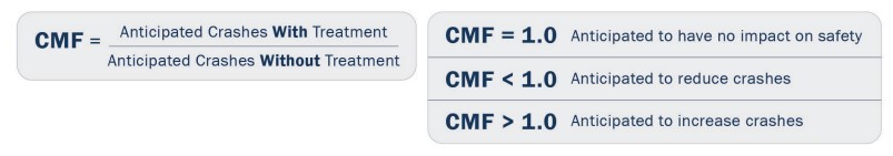
Figure 5-7: CMF Calculation
A CRF is similar to a CMF but stated as the percent reduction in crashes after a given countermeasure is implemented at a specific site. The CRF calculation based on the CMF is presented in .

Figure 5-8: Crash Reduction Factor Calculation
5.4.3 CMF Clearinghouse
CMFs are located on the CMF Clearinghouse website, which is a central, web-based repository of CMFs. This website is a searchable database maintained by FHWA with the intent of serving three roles related to the transportation safety field: to educate CMF users, house CMF data for use, and facilitate continued CMF research. The CMF Clearinghouse website includes search features for CMFs applicable to the various countermeasures under consideration. A link to the CMF Clearinghouse is available in
Appendix F, Section 3 – External References (Reference 2)
.All CMFs in the Clearinghouse are evaluated and rated using the defined star rating system. CMFs are given a star rating from one to five stars. The star rating indicates the reliability and quality of a CMF, with five stars being the most reliable. The star rating system considers various factors from the study research that produced the CMF. These factors include data used, study design, study methodology, sample size, statistical significance, and location(s) where the data was collected. An updated star rating system was developed and implemented in February 2021 as part of the NCHRP) 17-72 project. As a result, many CMFs received a new star rating based on the updated evaluation criteria. CMF summary reports printed prior to February 2021 may contain star ratings that differ from their current star rating. Additional information about the star rating system’s evaluation criteria and the changes to the evaluation criteria are on the CMF Clearinghouse website.
Whenever possible, only CMFs with a star rating of three or higher may be used in analysis. If the best available CMF has a star rating lower than three, it can only be used if accepted by the TxDOT project manager assigned to approve the completed analysis. A CMF’s ID number and star rating is suggested to be documented if used for safety analysis.
5.4.4 Selecting CMFs
Special attention is necessary when selecting CMFs for use in safety analysis to make sure that the practitioner is selecting appropriate CMFs. The primary goal is to select a CMF that was developed under the same (or very similar) conditions as the location for which it is being applied. When selecting CMFs, consider the following characteristics:
- Countermeasure type;
- Crash type;
- Crash severity;
- Roadway or intersection type;
- Area type (rural vs. urban);
- AADT ranges;
- Prior conditions; and
- Similarity to locality where data is used
If multiple CMFs are available and appear to be similar or equally applicable, it is suggested that the following items related to the quality of the CMFs are reviewed to determine the best possible match:
- Star rating;
- Score details; and
- Age of data or study
When selecting CMFs for use in analysis from the CMF Clearinghouse, the CMF IDs are recommended to be documented, and the CMF detail summary page can be provided. This information can be saved as a PDF and included as an appendix or attachment to the analysis documentation.
It is critical that sound engineering or professional judgment be used when selecting CMFs. Additional guidance on selecting CMFs is available in the following link:
Appendix F, Section 3 – External References (Reference 3)
.5.4.5 Applying Multiple CMFs
In many cases, the application of multiple safety-related improvements results in greater crash reduction benefits. This results in the possibility of multiple CMFs being applicable. The interaction between various safety treatments is complicated and can make it difficult to determine the true effectiveness of multiple treatments when used together. This is because CMFs are not always independent of one another, and it is possible to overestimate or underestimate the potential for crash reduction when applying the effects of multiple CMFs. A CMF is considered independent of another CMF if there is no overlap in their crash type and/or crash severity. For example, the installation of a pedestrian signal would be relatively independent of the installation of a left-turn phase at an adjacent intersection, because one addresses pedestrian-vehicle crashes while the other addresses left-turn opposite-direction crashes. An example of overlapping or non-independent CMFs would be multiple treatments focused on reducing nighttime crashes or multiple treatments focused on reducing run-off road crashes.
When applying multiple treatments, no more than three CMFs can be applied because it may overestimate the reduction of crashes. The following subsection provides an overview of four different methods that can be considered when applying multiple CMFs.
5.4.5.1 Dominant Effect Method
The dominant effect method applies the CMF for only the most effective treatment. The most effective treatment is the treatment with the lowest CMF value. This method is intended to be the simplest and most conservative approach. Typically, this method would be applied when the applicable CMFs are not independent of one another and have extreme overlap in the crash type and/or severity that are affected. The primary limitation of this method is that it is likely to underestimate the combined treatment effect if the additional treatments also improve safety.
5.4.5.2 Additive Effects Method
The additive effects method adds the effects of the CMFs together and presumes that the CMFs are independent and do not have overlapping effects. The following is an example of how to calculate the combined CMF value for the additive effects method:
CMF
= 1 − 1 [(1 − Combined
CMF
) + (1 − 1
CMF
) + (1 − 2
CMF
)]3
The primary limitation to this approach is the possibility that the combined effects may exceed 100 percent reduction in crashes or a CMF value less than zero.
5.4.5.3 Multiplicative Method
The multiplicative method estimates the combined effect of the various treatments being applied. Individual CMF values for each treatment are multiplied together to determine a combined CMF value. This is the most common method used at this time because it is identified in the HSM. The following is an example of the multiplicative method:
CMF
= Combined
CMF
× 1
CMF
× 2
CMF
3
The primary limitation of this method is that it is likely to either underestimate or overestimate the combined effects of the overall safety treatments if their effects are not independent of one another. This method can only be applied when it is presumed that all the CMFs are independent and there is no overlap.
5.4.5.4 Dominant Common Residuals Method
The dominant common residuals method is similar to the multiplicative method, except that the CMFs are non-independent of one another or slightly overlapping. The combined effect of the various treatments being applied is calculated by multiplying the individual CMF values together for each countermeasure and then raising that value to the power of the most effective or lowest CMF value. The following is an example of how the dominant common residuals method’s combined CMF value is calculated:
CMF
= (Combined
CMF
× 1
CMF
× 2
CMF
)3
CMF
1
This method is more conservative than the multiplicative method, but it is not appropriate for CMFs with values greater than 1.0 or if the most effective treatment has a CMF value greater than 1.0. A combined CMF value that is raised to a power greater than 1.0 intensifies the effects of the combined CMF rather than dampening its effects.
5.4.5.5 Examples of Applying Multiple CMFs
provides examples of the various methods outlined in this section of the manual related to the various methods for applying multiple CMFs. The hypothetical CMF values of 0.95, 0.65, and 0.80 were used in the example calculation table.
Method | Calculations | Resulting CMF Value |
|---|---|---|
Dominant Effect | CMF = 0.65 | 0.65 |
Additive Effects | CMF = 1 − [(1 − 0.65) + (1 − 0.80) + (1 − 0.95)]Combined | 0.40 |
Multiplicative | CMF = 0.65 × 0.80 × 0.95Combined | 0.494 |
Dominant Common Residuals | CMF = (0.65 × 0.80 × 0.95)Combined 0.65 | 0.632 |