3.2 Existing Traffic Volumes
Existing traffic volumes are the foundation of traffic forecasts. See
Chapter 2
for information on obtaining existing traffic volumes. It is recommended that existing traffic volumes are analyzed to extract traffic data factors and processed to provide consistent traffic forecasts. It is recommended that seasonal variation, historical factors, peak hour/period selection, outliers/disruptive events, balancing, and post processing be considered when using existing traffic volumes. TxDOT’s STARS II provides traffic volumes that are annualized to AADT. AADT estimates the mean traffic volume at a given location along a roadway across all days for a year. This data is used for both existing analysis and forecasting traffic volumes. Data, such as, the 30th highest hourly volume (K-factor), directional distribution (D-factor), percent trucks (T-factor), ADT, Design Hourly Volume (DHV), and vehicle classification can be obtained from STARS II. A graphic of the 30th highest hourly volume is shown in .
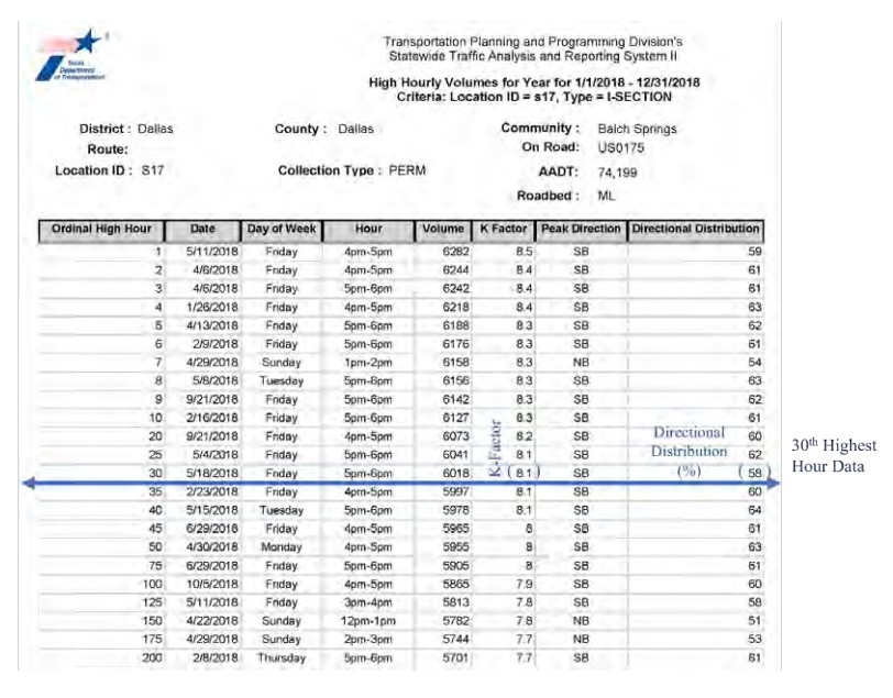
Figure 3-1: 30th Highest Hourly Volume
3.2.1 Traffic Data Factors
Common traffic data factors include the Kfactor, D-factor, and T-factor. The K-factor is the 30th highest hourly volume and is presented as a percentage of the ADT. The D-factor is the directionality of the 30th highest hourly volume of traffic. It is expressed as a percentage of the 30th highest hourly volume. The T-factor is the total percentage of single-unit trucks and multiunit combination trucks. TxDOT uses vehicle classification data and overall traffic volumes to determine the T-factor. TxDOT uses this data to develop Equivalent Single Axle Load (ESAL) calculations for pavement design. Traffic data factors are obtained from STARS II.
3.2.2 Seasonal Factors
AADT is calculated using a volume count, axle factor, and seasonal factor. The seasonal factor measures the amount by which monthly traffic volume is above or below the annual average. Calculating the AADT allows direct comparison of short term traffic counts collected throughout the year
3.2.3 Historical Factors
Historical growth rates are developed by calculating traffic growth rates between past years at multiple locations within and near the study area. It is suggested that historical growth rates are developed for as many years as there is available data. It is suggested that regression analysis be performed on historical counts to determine an average linear growth rate. Historical growth factor is determined based on the average growth rate. Check traffic data to assess whether it is necessary to exclude any outlier data from the analysis and document accordingly. An example of the historical growth rate calculation is provided in
Appendix D, Section 4 – Regression Calculations
.3.2.4 Peak Hour/Period Selection
For roadway segments, 24-hour counts can be used to determine the time of day (e.g., AM, midday, or PM) peak hour or peak period. For intersections, segment counts or TMCs can be used to determine the peak hour or peak period. The peak hour is the hour in which the sum of vehicle volume during four consecutive 15-minute count intervals is the highest. shows an
example
of 24-hour traffic counts for a corridor, which can be used for AM and PM peak hour selection. This figure shows that the AM peak hour probably occurs sometime between 7:00am and 9:00am and that the PM peak hour probably occurs sometime between 3:30pm and 5:30pm. Typically, the morning and evening peaks are used for analysis. Unique circumstances could necessitate the analysis of a midday peak, weekend peak, or other atypical peak. This is an important consideration near malls, commercial corridors, stadiums, schools, and unique land uses because these locations may cause sporadic or irregular traffic patterns. In oversaturated conditions, peak spreading may occur and necessitate a peak period selection rather than a peak hour. It is suggested that selection of peak hour/period be documented.
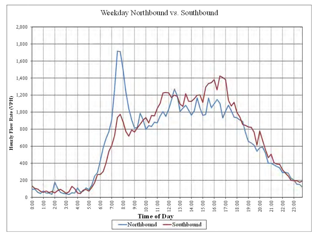
Figure 3-2: Peak Hour/Period Selection Using Count Data
3.2.5 Disruptive Events
Existing traffic volumes can be affected by disruptive events. During disruptive events (such as the COVID-19 pandemic or inclement weather conditions), data collected may need adjustment to account for anticipated impacts of the disruption and to remove outliers.
Options for obtaining data during a disruptive event vary based on the disruption type, duration, data availability, and data limitations. If data is less than two years old and was not collected during a recent disruptive event it can be used as is. In other situations, lack of recent counts could create the need for counts to be grown with historical growth rates or validated by big data. Big data uses geolocation services to sample the number of users on a transportation facility and their movements.
Figure 3-3
shows a decision tree to help decide what method to use for traffic analysis.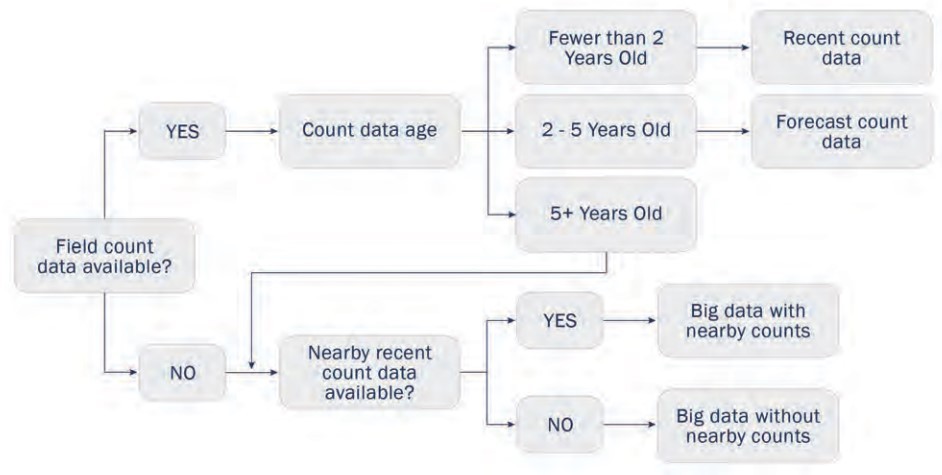
Figure 3-3: Traffic Volume Derivation Methodology Decision Tree for Disruptive Events
3.2.6 Traffic Balancing
Traffic volumes are considered balanced when no volume discrepancies exist between adjacent locations in the project area. Balancing typically begins at one extremity of the project and ends at the other extremity of the project until all discrepancies have been flushed out of the network. Include high-volume driveways that serve high-density developments. Balance base year volumes and traffic forecasts. It is recommended that counts are balanced before analysis begins, though there may be circumstances where counts will not balance due to land use and special traffic generators. Before balancing begins, round counts to the nearest determined interval unit. For standard rounding conventions, see
Section 3.2.7
about post processing.3.2.7 Post Processing
Traffic volumes are typically rounded up to the nearest 100 unit (e.g., vehicle, truck) but are rounded up to the nearest 50 if the traffic volumes are between 100-200. Traffic volumes are typically rounded up to the nearest 10 or 25 if traffic volumes are under 100. However, using numbers under 100 may cause balancing issues. It is recommended that identical volumes be rounded to the same value. Additionally, identical volumes typically result in the same values when forecasted.
3.2.8 Validation
Validate existing volumes by checking against field observations, historical traffic counts, traffic volumes from adjacent projects, adjacent land use, and the capacities defined in the HCM. and show the capacities of basic freeway segments, multilane highway segments, and ramps based on the HCM 7th Edition. If there are discrepancies between data points, validate with additional data sources.
Free Flow Speed (mi/h) | Capacity (pc/h/In) | |
|---|---|---|
Basic Freeway Segment | Multi-Lane Highway Segment | |
75 | 2,400 | N/A |
70 | 2,400 | 2,300 |
65 | 2,350 | 2,300 |
60 | 2,300 | 2,200 |
55 | 2,250 | 2,100 |
50 | N/A | 2,000 |
45 | N/A | 1,900 |
Ramp Free Flow Speed (mi/h) | Capacity (pc/h) | |
|---|---|---|
Single-Lane Ramps | Two-Lane Ramps | |
>50 | 2,200 | 4,400 |
>40-50 | 2,100 | 4,200 |
>30-40 | 2,000 | 4,000 |
>=20-30 | 1,900 | 3,800 |
<20 | 1,800 | 3,600 |