Section 3: TIA Example Problems
Trip Generation
Site-generated traffic estimates are determined through a process known as trip generation. Rates and equations are applied to the proposed land use to estimate traffic generated by the development during a specific time interval. The acknowledged source for trip generation data is the 11th edition of
Trip Generation Manual
published by the Institute of Transportation Engineers (ITE). ITE has established trip data in nationwide studies of similar land uses. The following example poses a case study for calculating trip generation at a proposed site.Assume you are dealing with a development that contains 300 dwelling units of single family detached housing. Trip generation must be calculated using either the average rates or equations provided on the data plots in the latest edition of the ITE
Trip Generation Manual
.The ITE
Trip Generation Handbook
considers the following criteria for calculating trip generation based on either the equation or the rate.- The number of data points available
- Whether the size of the land use is within the provided data extremes
- Whether the fitted curve equation is provided on the data plots
- The R2 value of the data
- The standard deviation of the data.
In this case, because the data plots for single family detached housing have a fitted curve equation provided, and because each study scenario has over 20 data points available, the fitted curve equation is used for trip generation calculations. Further information on deciding between average rate and the fitted curve equation is available in
Section 16.3.3 Analysis Assumptions
or in the ITE Trip Generation Handbook
Chapter 4, “Trip Generation Manual Data”.The following equation represents the number of weekday one-way vehicle trips for a single-family detached housing land use.
Ln(T) = 0.92 Ln(X) + 2.68
X represents the number of dwelling units of the proposed development, while T represents the number of vehicle trip ends generated by the development.
After inputting the number of dwelling units (300) and solving for T, it is calculated that the development generates approximately 2,772 daily one-way trips.
Similarly, the following equation represents the number of trips ends during the AM peak hour of adjacent street traffic.
Ln(T) = 0.91 Ln(X) + 0.12.
Once again, after inputting the number of dwelling units (300) and solving for T, this scenario yields 202 total AM peak hour trips.
The number of inbound and outbound vehicle trips can then be determined by applying the directional distribution percentages, which are also provided by ITE. In this case 25% of vehicles enter, and 75% of vehicles exit the development during the AM Peak hour of adjacent street traffic.
Inbound vehicles = 202 * (0.25) = 51
Outbound vehicles = 202 – 51 = 151
This same process is repeated for the PM peak hour of adjacent street traffic. The weekday daily, AM peak hour, and PM peak hour one-way vehicle trips are summarized in
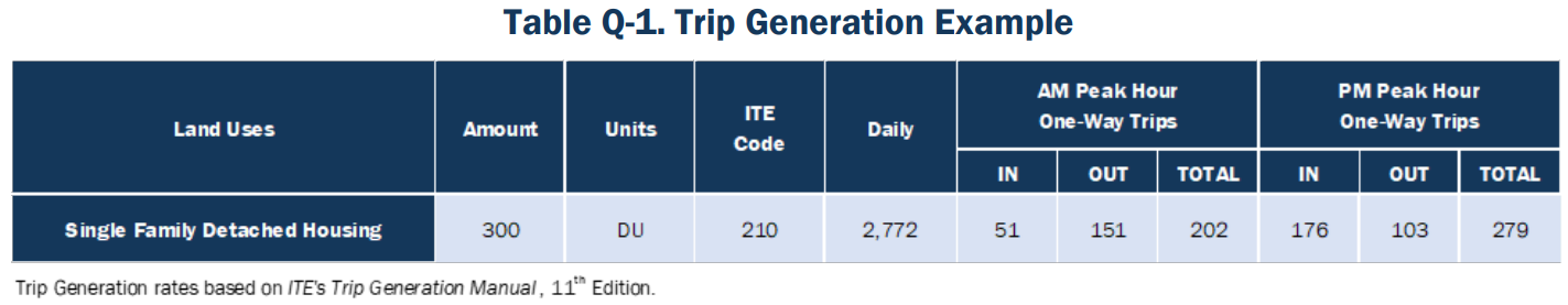
Because the maximum peak hour trip generation in this case is 279 veh/hr, this would classify as a category 1 TIA as shown in section
16.2.1 TIA Categories, Table 16-1
.Estimating Mixed-Use Trip Generation / Internal Capture Reduction
In cases when a development contains two or more complementary land uses, there is potential for interaction among those uses. This is referred to as “Internal Capture Trips”, where a reduction in the total generation of external trips is accounted for due to trips within the same development that do not touch the off-site street system. Additional information on Internal Capture is found in the ITE
Trip Generation Handbook
, Chapter 6 “Trip Generation for Mixed-Use Development”.Assume you are dealing with a development that contains 250 dwelling units of low-rise multifamily housing, 250,000 SF of office space, and 50,000 SF of retail space. Individual trip generation calculations for each land use are shown in
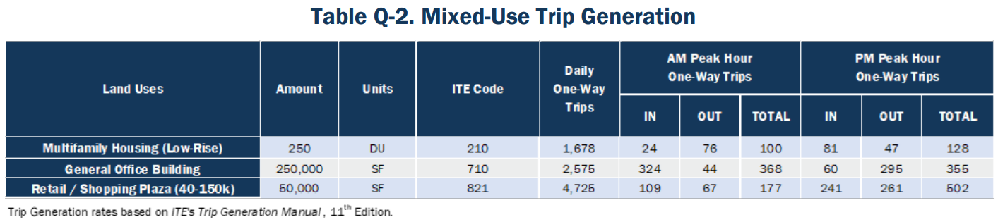
The following steps for calculating internal capture are provided in the ITE
Trip Generation Handbook,
Chapter 6.Step 1:
Determine whether methodology is appropriate for study site.
Step 2:
Estimate person trip generation for individual on-site land uses.Step 3:
Estimate proximity between on-site land use pairs.Step 4:
Estimate unconstrained internal person trip capture rates with proximity adjustment.Step 5:
Estimate unconstrained demand between on-site land use pairs.Step 6:
Estimate balanced demand between on-site land use pairs.Step 7:
Estimate total internal person trips between on-site land use pairs.Step 8:
Estimate total external person trips for each land use.Step 9:
Calculate overall internal capture and total external vehicle trip generation.Steps 1 & 2 have already been completed above. Step 3, proximity adjustment, was not done in this problem since no distinction was made between vehicle and non-vehicle trips. However, this should not impact the distinction between internal trips and external trips.
Steps 4-9 are automatically calculated with the internal capture spreadsheet tool provided on the ITE website:
Using this tool, you plug in the trip generation values for each land use into Table 1-A and Table 1-P. The resulting computations summary table (Table 5-A and Table 5-P) shows the new external vehicle trips after the internal capture reduction has been applied. The AM and PM peak hour trips for the mixed-use development after internal capture has been applied are shown in
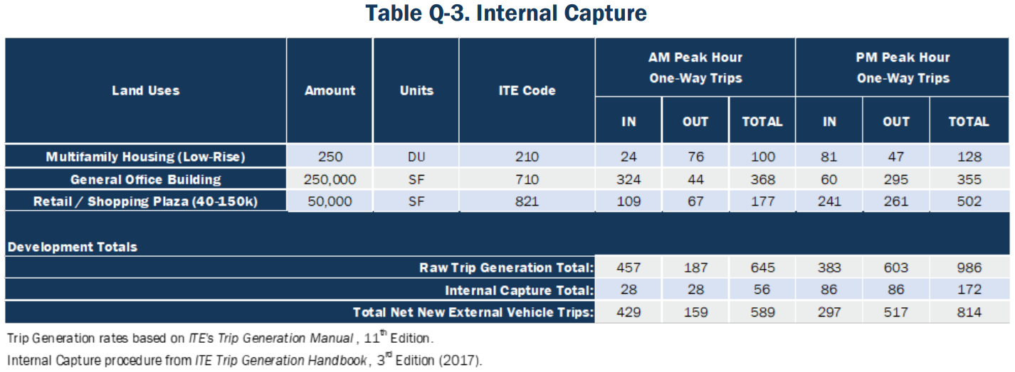
Because the maximum peak hour trip generation in this case is 814 veh/hr, this would classify as a category 2 TIA as shown in section
16.2.1 TIA Categories, Table 16-1
.Additional detail on each step of the internal capture estimation process is available in the ITE
Trip Generation Handbook
, Section 6.5 “Process for Estimating Mixed-Use Trip Generation”.Trip Distribution and Assignment
Trip Distribution
Trip distribution refers to the origins and destinations of site-generated trips from the proposed development.
Assume you are dealing with a multifamily development. After evaluation of the existing counts, traffic percentages entering and exiting the study area can be calculated by dividing the number of traffic to/from each direction with the total traffic at all approaches along the edges of the study area.
Based on existing traffic counts, the following traffic distribution percentages are shown:
- 45% of existing traffic travels in or out from the south (Road 3 and Main Steet)
- 55% of existing traffic travels in or out from the north (Road 1, Road 2, and Main Street)
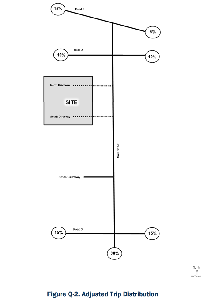
The distribution percentages are displayed in
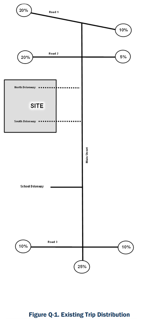
Existing traffic patterns should be used as a starting point for determining trip distribution percentages. However, the existing traffic pattern percentages should be altered based on engineering judgement and context dependent characteristics. These characteristics may include:
- The land use of the development
- The street system characteristics
- Nearby central business districts or employment centers
In this case, let’s say Road 1 and Road 2 connect to rural highways to the north while Main Street and Road 3 connect to employment centers and denser development to the south. It would make more sense for the majority of users of the multifamily development to travel south towards employment centers rather than to the rural highway to the north. Additionally, Road 1 and Road 2 intersect at a point approximately 3,000 feet east of the study area. This would mean that vehicles are more likely to travel along Road 2 when coming from the east rather than on Road 1, since it provides a more direct route to the development.
The adjusted trip distribution percentages based on the provided context are shown in As always, engineering judgement should be exercised when developing distribution percentages according to the context of your development scenario. Distribution results are typically reviewed and approved by TxDOT or the applicable city/county.
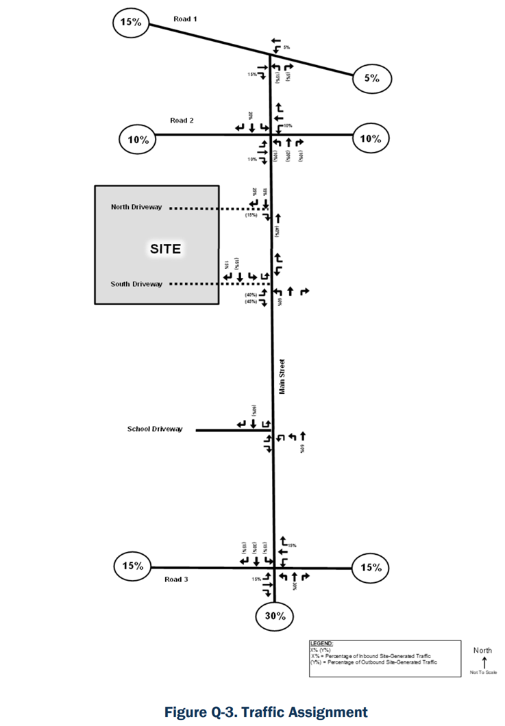
Traffic Assignment
Whereas trip distribution refers to the origins and destination of site generated trips, traffic assignment refers to the specific routes that the trips will take along the roadway network and into the site driveways. In this case, the following assumptions are made:
- Drivers will tend to use the first available driveway when reaching the development.
- No northbound left or eastbound left turns are made at the position of North Driveway, due to there being no median opening at this access point.
- More drivers will use South Driveway to exit the development, due to a median opening on Main Street allowing outbound vehicles to turn left towards the north. Additionally, it is also the closest driveway to the south which is where the majority of vehicles are traveling from.
The corresponding inbound and outbound traffic assignment is shown in . Once again, engineering judgement should be exercised to appropriately assign the traffic according to site specific characteristics of the development.
Background Site Traffic Assignment
In some cases, future developments near the study area are slated to open during the period of analysis. These sites need to be included in the traffic analyses. As a result of this, traffic assignment for the corresponding background development must also be added to the surrounding roadway network. If a TIA has been completed for the site, the traffic assignment reported in that TIA should be used, when a TIA is not available traffic assignment should be completed in a similar methodology as site trip distribution and traffic assignment.
Take the case shown above, but now with an additional background development directly east of the site, across Main Street. The background development contains an additional right-in, right-out, driveway on its northern side that is not within the boundaries of the studied intersections of the original development. This driveway from the background development is not studied and not shown on the figure. However, it will be necessary to assign traffic that will travel through the studied roadway network, as well as to the background driveway that is directly east of South Driveway.
The corresponding traffic assignment for the background development is shown in .
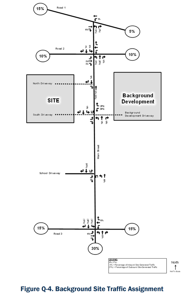
Likewise, any additional background developments must also have their own corresponding traffic assignment along the surrounding roadway network.
Projected Traffic
Determining Background Growth Rates
When analyzing future conditions, existing traffic is grown using compound growth rates extended to the future study years specified in the scope.
The annual growth rate may be available from the city or MPO. When available, the annual growth rate can also be based on historical AADT information, where historical AADT data within the road network is averaged for at least the last five years of data. Historical AADT data may be available from the TxDOT Traffic Count Database System linked in
Appendix Q, Section 4 – External References (Reference 1)
. shows a historical example data from the Traffic Count Database System, where the 24- hour volume column represents the AADT data for each year.
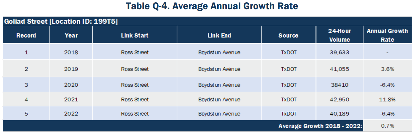
The annual growth rate is calculated by applying the following compound annual growth rate formula.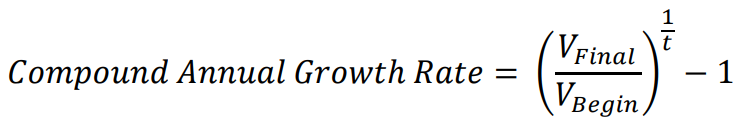
Where V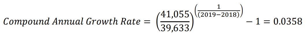
Final
and VBegin
represent the AADT data for each year, and t represents the number of years between each AADT data point. From 2018 to 2019, the compound annual growth rate is calculated as follows:Represented as a percentage, 0.0358 can be expressed as approximately 3.6%. This process is repeated for each of the five years of available data and an average is taken, in this case, the average growth rate was 0.7%.
In cases where 5 consecutive years of AADT data are not available, engineering judgement should be used to estimate the annual growth rate from the best available data points.
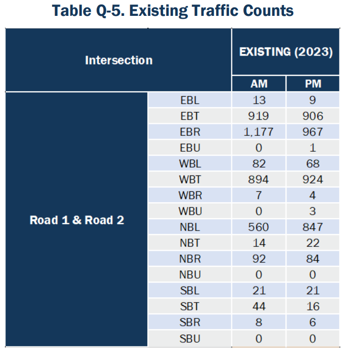
Future Background Growth
As mentioned earlier in this section, the calculated annual growth rate is used for future background traffic analysis, where existing traffic is grown according to the future study years specified in the scope. Take the existing intersection traffic counts shown in .
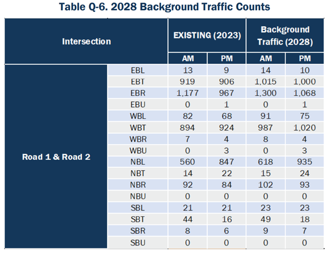
The traffic counts for each movement are grown by the compound growth rate using the following formula.
Where P represents the existing traffic, r represents the rate, and t represents the number of years that the traffic will be grown to. Let’s say you want to grow the AM traffic counts at the EBT movement at a rate of 2% for 5 years. After plugging in each value, the estimated future traffic is rounded to 1015.
Similarly, the same equation is applied to each traffic movement and displayed in .
This process is repeated for any other traffic counts that you wish to grow for any number of future study years.
Traffic Operations Analysis
Intersection Analysis Methodology
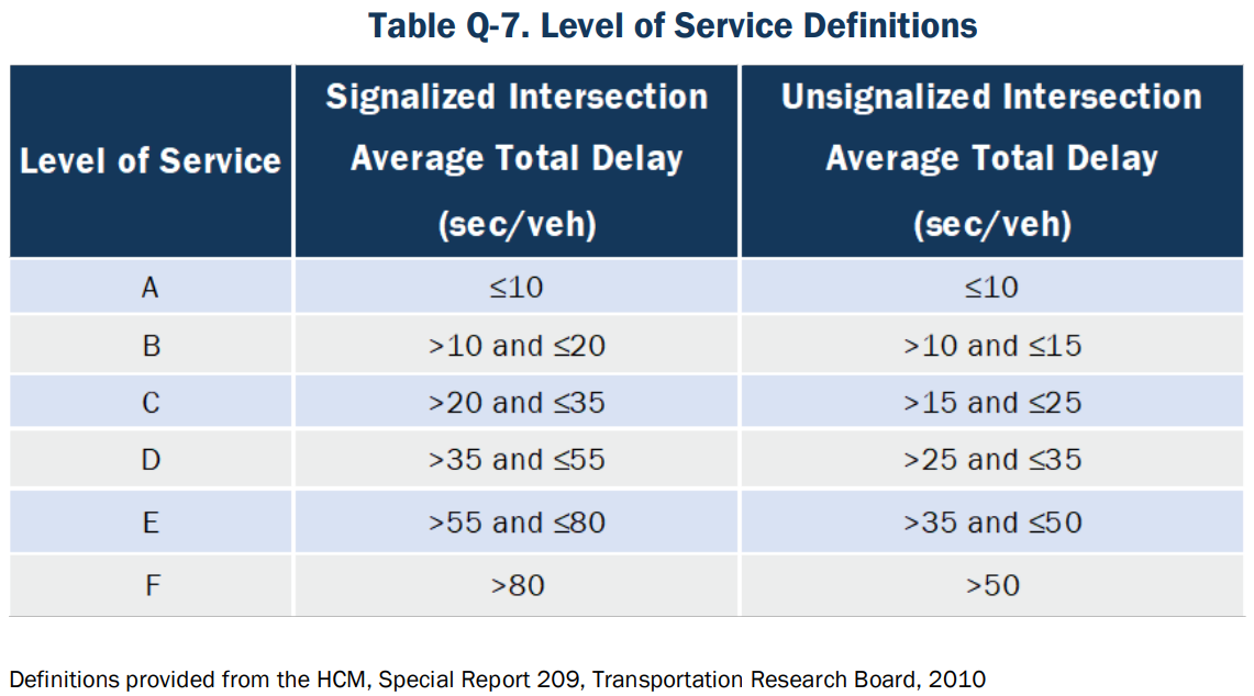
This section provides one example using HCM methodology for delay and Level of Service (LOS) to measure intersection operations. The level of detail required for intersection operations analysis may vary from project to project, may vary due to the TxDOT project manager, or due to applicable city / county requirements. This example is not meant to be exhaustive. The required intersection analysis for each project should be consulted with the appropriate authorities prior to beginning the study.
shows the definition of LOS for signalized and unsignalized intersections.
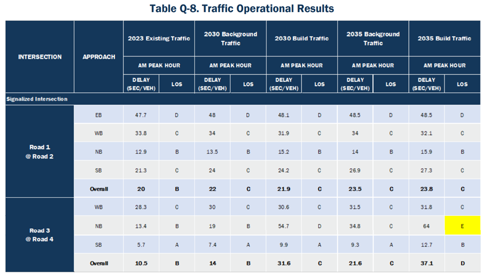
The synchro software was used to analyze the following two signalized intersections during the AM peak hour. Average delay and LOS are reported for each approach during existing, background, and buildout scenarios. The results are shown in . In this case, background traffic consists of existing traffic with added compound growth rates grown to 2030 and 2035, while build out traffic consists of background traffic combined with site generated traffic.
Build Versus No-Build Analysis
Intersection operations are analyzed for the following scenarios.
- Existing conditions
- Background (no-build)
- Build
Existing conditions are used as a baseline to compare the impact a development has on traffic operations during future conditions. Background (no-build) consists of existing traffic volumes grown with compound growth rates to the future study years. In this case, the future study years consisted of 2030 and 2035, therefore, traffic volumes were grown for seven and twelve years respectively. In cases where additional background developments are near the study area, site generated traffic from the proposed developments must also be added to the background traffic.
Build scenarios consist of the previously mentioned background traffic combined with sitegenerated traffic from the proposed development.
As shown in the table above, LOS E was reported in the northbound direction of Road 3 and Road 4 during the 2035 build scenario. The addition of site generated traffic caused the northbound delay at the intersection to increase from 34.8 sec/veh to 64.0 sec/veh, which caused the LOS to worsen from LOS C to LOS E. Assuming the threshold at this jurisdiction is to not have any approach drop below LOS D, a mitigation would be required at this intersection.
Other than the approach identified above, all other approaches register LOS D or better. Site generated traffic has little impact on delay, with all other approaches operating with acceptable delay times.
Mitigation
Where necessary, recommendations are required to mitigate impacts from the additional traffic generated by the development. Recommendations can include altering lane configurations and geometries of the intersection, optimizing signal timings, modifications to the traffic control at the intersection, or reducing the projects density. These changes are documented as mitigations, which are evaluated to improve intersection operations to an acceptable threshold set by varying project specific, TxDOT District, or city/county requirements.
In this case, due to the large delay present at the northbound approach on Road 3 and Road 4, mitigation will be required to improve the LOS at this intersection to an acceptable threshold. Because it is already signalized, traffic signal timing adjustments were recommended. lists Road 3 and Road 4 before and after traffic signal timing adjustments have been made.
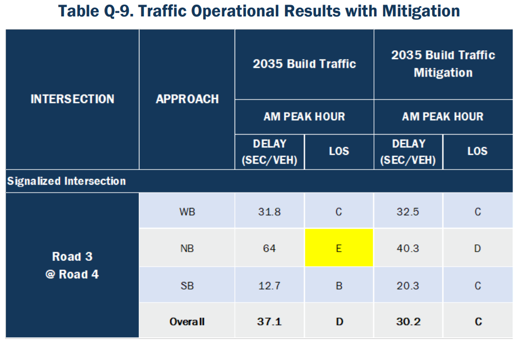
As shown, northbound delay at the intersection decreases from 64 sec/veh to 40.3 sec/veh, improving from LOS E to LOS D. Assuming that the acceptable LOS threshold is LOS D this approach now satisfies the necessary criteria after implementing the mitigation
Site Driveway Analysis
Access Connection Spacing
Access management guidelines for driveway spacing can be found in the TxDOT
Access Management Manual
(Appendix Q, Section 4 – External References ‘Reference 4’
). As per the Access Management Manual,
these standards are designed to enable the highway to function efficiently while at the same time providing reasonable access to development.Distance between access connections is measured along the edge of the traveled way from the closest edge of pavement to closest edge of pavement. Refer to Figure 2-1
Access Connection Spacing Diagram
on the TxDOT Access Management Manual
for more information.Take the following development and corresponding access connections shown in . Assume that Main Street in this case has a speed limit of 35 MPH.
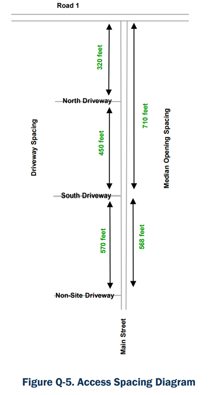
Minimum connection spacing criteria for State highways can be found on Table 2-2 of the TxDOT Access Management Manual. Access spacing at the development and corresponding TxDOT criteria is shown on below.
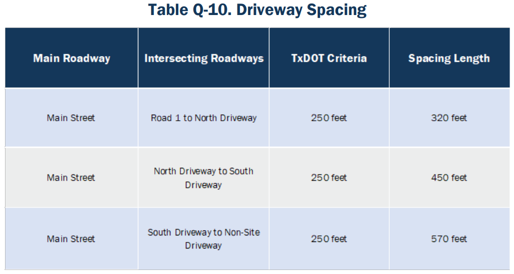
As shown, the development satisfies the required TxDOT driveway spacing criteria.
Other driveway spacing criteria along frontage roads is shown on Table 2-1 of the
Access Management Manual
. Engineering judgement should be exercised when deciding on the appropriate spacing criteria to use for your specific project.Additionally, shows median opening spacing on the proposed development. There is no official median opening spacing requirement per the TxDOT 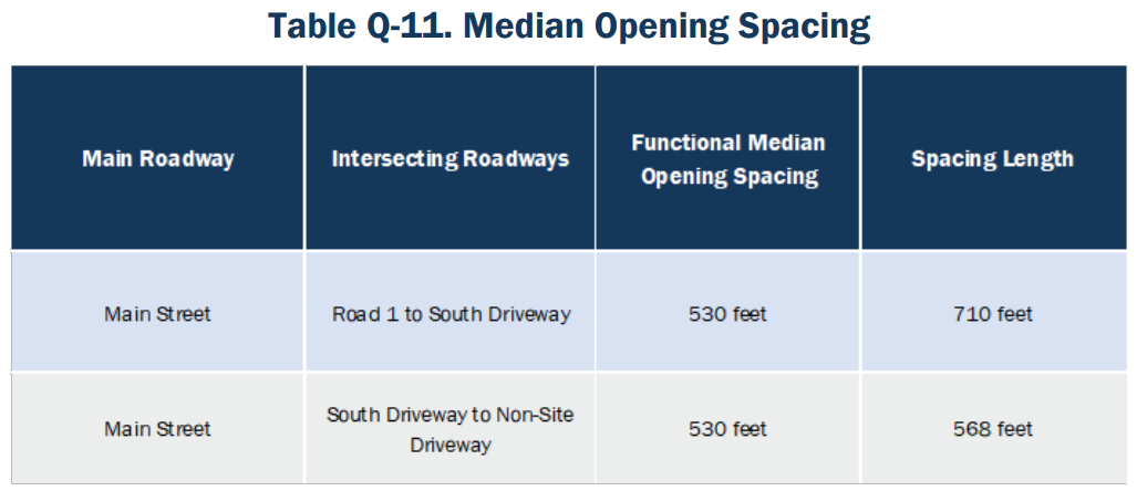
Access Management Manual
. However, median opening spacing is the minimum for normal TxDOT design left-turn lanes on both ends. The following table shows the median spacing of the proposed development along with the functional median opening spacing.Engineering judgement should be exercised when the development does not satisfy TxDOT access connection criteria. Additionally, a variance may be requested per the process shown in Chapter 2 of the TxDOT
Access Management Manual.
Auxiliary Lane Analysis
Where justified, the addition of right-turn deceleration lanes can help inbound turning vehicles separate from the through traffic, avoiding conflicts and smoothing traffic flow. TxDOT has identified right-turning volume thresholds where right-turn lanes are justified. Assume the following peak hour right turn volumes into the development in .
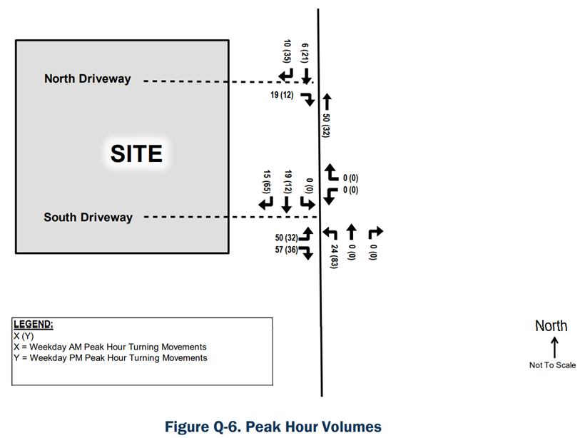
shows the driveway locations with right-turn driveway access to the site, and how they compare with the TxDOT right turn volume threshold per the Access Management Manual.
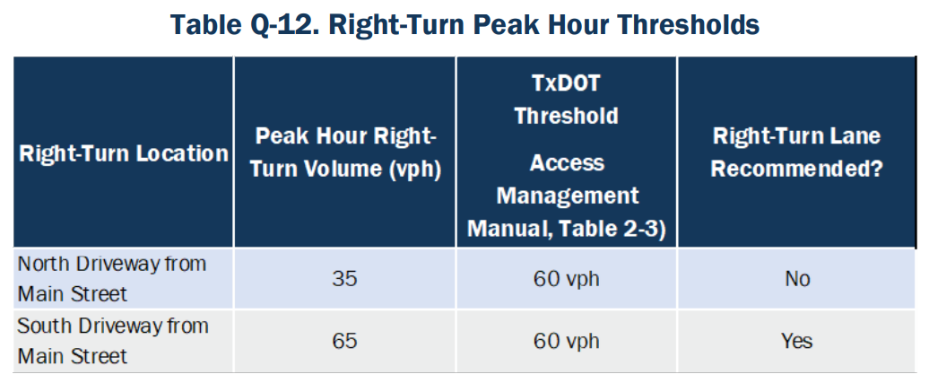
In this case, a right turn lane is not recommended at North Driveway, while it would be recommended at South Driveway.
Per TxDOT
Access Management Manual
(Table 2-3), Left turn deceleration lanes are justified at median openings that provide direct access to the proposed development wherever left turns are permitted. Therefore, in this case, a left turn deceleration lane is recommended at the median opening at South Driveway.As always, engineering judgement must be exercised when recommending turn lanes at developments.