15.4 Performance Measurement
15.4.1 Overview
For discussion of MOEs see
Section 15.3.2
.Chapter 11 of the HCM 7th Edition builds on the basic freeway analysis presented in the HCM and provides a methodology for evaluating a freeway’s travel time reliability over a multiday or multi-month reliability reporting period (RRP) and under a variety of conditions, such as lane closures, traffic incidents, or periods of inclement weather.
Freeway reliability refers to the distribution or variability of travel times of trips through an entire freeway facility over a period of time, typically one year. Travel time variation may be caused by recurring variations in demand by hour of day, day of week, and month of year, which are generally predictable in distribution. Travel time variation may also be caused by less predictable non-recurring variations in demand or available roadway capacity.
The methodology estimates the impacts of recurring and nonrecurring congestion on travel time variability and can also estimate the impacts that TSMO and TDM strategies have on travel time and travel time variability. Many TSMO and TDM strategies target reducing congestion and delays associated with the nonrecurring factors described below and, as a result, reducing travel time variation. Nonrecurring factors that impact travel time include:
- Severe weather that reduces speeds and capacity and influences demand;
- Incidents that reduce capacity;
- Work zones that reduce capacity and influence demand; and
- Special events that produce temporary spikes in traffic demands, which may be recurring or nonrecurring
HCM freeway reliability analysis methods may be used to assess the influence of TSMO and Active Transportation and Demand Management (ATDM) projects on a freeway and the impacts of recurring and nonrecurring events that occur on the facility. The reliability analysis allows individual TSMO and ATDM projects, as well as any combination of projects, to be analyzed under a variety of freeway conditions. The analysis determines the full range of capacity under any condition, combination of conditions, and implemented transportation improvements.
For additional information and case studies on TSMO, ATDM, and performance measurement see
Appendix P, Section 2 – External References (References 5,6, and 7)
.15.4.2 Methodology
The freeway reliability analysis relies on the freeway facilities core methodology presented in Chapter 10 of the HCM 7th Edition, which is described in
Chapter 9
of this manual. A base dataset is used to develop a base scenario, which is then adjusted to create a variety of different scenarios that represent the range of actual freeway capacity and facility demand as conditions on the facility change. The travel time distribution produced from the results of each scenario’s travel time calculations may be used to determine reliability performance measures of the analyzed freeway segment. Adjustments associated with TSMO and ATDM projects can then be applied to appropriate scenarios to assess the impacts of the projects. shows the freeway reliability analysis methodology framework as shown in the HCM.
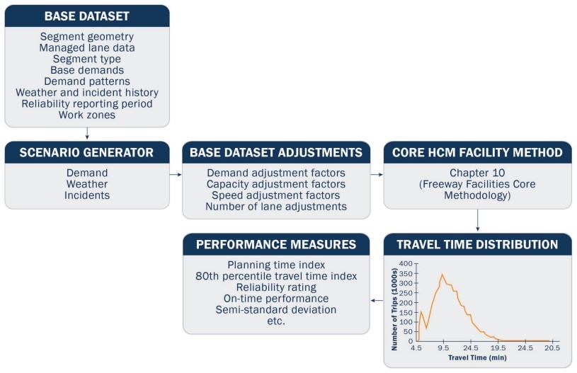
Figure 15-1: Freeway Reliability Methodology Framework
15.4.3 Scenario Generation
The freeway capacity analysis analyzes 15- minute periods of extended lengths of freeway comprised of continuous connected basic freeway, weaving, merge, and diverge segments. A base dataset provides all the necessary input data for the freeway facilities core methodology, including the facility’s geometry, free-flow speeds, lane patterns, segment types, and base demand volumes. This initial freeway capacity analysis produces a base scenario model for the freeway reliability analysis.
A freeway’s performance is typically analyzed under different conditions to get a more accurate picture of the facility’s operations throughout the study period. Therefore, after a base scenario model is developed, a set of scenarios is created by modifying the base dataset inputs and applying adjustments, including CAFs, speed adjustment factors (SAFs), and demand adjustment factors (DAFs), associated with various factors that impact freeway capacity, such as weather events, traffic incidents, and work zones. These scenarios are generated to reflect conditions that a freeway facility experience during the RRP. Each scenario represents a single study period with adjusted demand and capacity variations specific to that scenario.
The default number of scenarios generated in a typical freeway reliability analysis, without considering weekends, is 240. This value was obtained by creating four replications of each weekday-month demand combination. Analyzing multiple replications of each weekday-month combination confirms the presence of a large sample of weather and incident events. The number of scenarios can be fewer or greater, depending on the scope of the analysis, range of factors, and the target performance measures.
15.4.4 Factors Affecting Travel Time Reliability
The factors that affect travel time reliability tend to adjust either the demand placed upon a facility, the effective available capacity of the facility, or the base travel speed that vehicles travel at while using the facility. Each factor is described in greater detail below.
15.4.4.1 Traffic Demand
Traffic demand fluctuates both across days within the week and across months of the year. Daily and weekly fluctuations can be caused by work schedules, typical working business hours, and other factors. Monthly fluctuations can be caused by seasonal activities, such as sporting events, recreational activities, and school session schedules. Traffic demand also fluctuates across the year due to holidays, religious festivals, fairs, concerts, and other special events.
The base freeway analysis scenario accounts for traffic demand variation for different hours of a given day. To account for day-to-day traffic demand variability in the generation of multiple scenarios, the traffic demands for the analysis period are calibrated by applying a demand multiplier based on the day of week and month combination. The demand multiplier is a ratio of the day-month combination daily facility demand to the daily facility demand for a reference period. These factors are first used to adjust demand data used in the base scenario to what may be expected in terms of demand for the reference period. A second adjustment changes the demand of the reference day-and-month combination to the expected demand for any other day-month combination analyzed as part of the RRP. and provide default demand ratios for urban and rural freeways, respectively, with ratios shown relative to traffic demand on a Monday in January. These values can be supplemented by locally collected demand factors if they are available.
15.4.4.2 Weather Events
The base scenario assumes ideal driving weather conditions; clear, no precipitation, and high visibility. However, different weather conditions have a wide range of impacts on the capacity of a freeway and the free flow travel speed, depending on the severity of the weather event. Inclement weather, such as snow, rain, or fog, can degrade driving conditions by creating slick roads, flooding, or limiting visibility. These conditions may result in reduced roadway capacity and reduced free flow speeds.
CAFs and SAFs for weather events are applied to scenarios across a RRP based on the probability of a weather event’s occurrence during a given month in the freeway location. For example, if historical weather trends indicate for a given month that heavy rain events occur across ten percent of days, then the relevant AFs for that weather event can be applied at random to ten percent of the scenarios analyzed for that month. This methodology can be repeated for all types of weather. The 11 weather categories consist of one non-severe weather category that includes all weather conditions that generate no capacity, demand, or speed adjustments, and ten categories of severe weather events that have been shown to reduce capacity by at least four percent. CAFs are shown in and SAFs are shown in .
Month | Day of Week | ||||||
|---|---|---|---|---|---|---|---|
Monday | Tuesday | Wednesday | Thursday | Friday | Saturday | Sunday | |
January | 1.00 | 1.00 | 1.02 | 1.05 | 1.17 | 1.01 | 0.89 |
February | 1.03 | 1.03 | 1.05 | 1.08 | 1.21 | 1.04 | 0.92 |
March | 1.12 | 1.12 | 1.14 | 1.18 | 1.31 | 1.13 | 0.99 |
April | 1.19 | 1.19 | 1.21 | 1.25 | 1.39 | 1.20 | 1.05 |
May | 1.18 | 1.18 | 1.21 | 1.24 | 1.39 | 1.20 | 1.05 |
June | 1.24 | 1.24 | 1.27 | 1.31 | 1.46 | 1.26 | 1.10 |
July | 1.38 | 1.38 | 1.41 | 1.45 | 1.62 | 1.39 | 1.22 |
August | 1.26 | 1.26 | 1.28 | 1.32 | 1.47 | 1.27 | 1.12 |
September | 1.29 | 1.29 | 1.32 | 1.36 | 1.52 | 1.31 | 1.15 |
October | 1.21 | 1.21 | 1.24 | 1.27 | 1.42 | 1.22 | 1.07 |
November | 1.21 | 1.21 | 1.24 | 1.27 | 1.42 | 1.22 | 1.07 |
December | 1.19 | 1.19 | 1.21 | 1.25 | 1.40 | 1.20 | 1.06 |
Note: Ratios represent demand relative to a Monday in January
Source: HCM 7th Edition
Month | Day of Week | ||||||
|---|---|---|---|---|---|---|---|
Monday | Tuesday | Wednesday | Thursday | Friday | Saturday | Sunday | |
January | 1.00 | 1.96 | 1.98 | 1.03 | 1.22 | 1.11 | 1.06 |
February | 1.11 | 1.06 | 1.09 | 1.14 | 1.35 | 1.23 | 1.18 |
March | 1.24 | 1.19 | 1.21 | 1.28 | 1.51 | 1.37 | 1.32 |
April | 1.33 | 1.27 | 1.30 | 1.37 | 1.62 | 1.47 | 1.41 |
May | 1.46 | 1.39 | 1.42 | 1.50 | 1.78 | 1.61 | 1.55 |
June | 1.48 | 1.42 | 1.45 | 1.53 | 1.81 | 1.63 | 1.57 |
July | 1.66 | 1.59 | 1.63 | 1.72 | 2.03 | 1.84 | 1.77 |
August | 1.52 | 1.46 | 1.49 | 1.57 | 1.86 | 1.68 | 1.62 |
September | 1.46 | 1.39 | 1.42 | 1.50 | 1.78 | 1.61 | 1.55 |
October | 1.33 | 1.28 | 1.31 | 1.38 | 1.63 | 1.47 | 1.42 |
November | 1.30 | 1.25 | 1.28 | 1.35 | 1.59 | 1.44 | 1.39 |
December | 1.17 | 1.12 | 1.14 | 1.20 | 1.43 | 1.29 | 1.24 |
Note: Ratios represent demand relative to a Monday in January
Source: HCM 7th Edition
Weather Type | Weather Event Definition | Capacity Adjustment Factors | ||||
|---|---|---|---|---|---|---|
55 mi/h | 60 mi/h | 65 mi/h | 70 mi/h | 75 mi/h | ||
Medium rain | >0.10-0.25 in./h | 0.94 | 0.93 | 0.92 | 0.91 | 0.90 |
Heavy rain | >0.25 in./h | 0.89 | 0.88 | 0.86 | 0.84 | 0.82 |
Light snow | >0.00-0.05 in./h | 0.97 | 0.96 | 0.96 | 0.95 | 0.95 |
Light-medium snow | >0.05-0.10 in./h | 0.95 | 0.94 | 0.92 | 0.90 | 0.88 |
Medium-heavy snow | >0.10-0.50 in./h | 0.93 | 0.91 | 0.90 | 0.88 | 0.87 |
Heavy snow | >0.50 in./h | 0.80 | 0.78 | 0.76 | 0.74 | 0.72 |
Severe cold | <-4°F | 0.93 | 0.92 | 0.92 | 0.91 | 0.90 |
Low visibility | 0.50-0.99 mi | 0.90 | 0.90 | 0.90 | 0.90 | 0.90 |
Very low visibility | 0.25-0.49 mi | 0.88 | 0.88 | 0.88 | 0.88 | 0.88 |
Minimal visibility | <0.25 mi | 0.90 | 0.90 | 0.90 | 0.90 | 0.90 |
Non-severe weather | All conditions not listed above | 1.00 | 1.00 | 1.00 | 1.00 | 1.00 |
Note: Speeds given in column heads are free-flow speeds.
Source: HCM 7th Edition
15.4.4.3 Traffic Incidents
The base scenario assumes the freeway is operating at full capacity with no traffic incidents or closures. However, the impacts of a traffic incident on freeway operations can vary depending on the severity of the incident and the extent of the resulting closure. Incidents typically cause shoulder or lane closures, as disabled vehicles block the roadway, and vehicles passing incidents tend to drive slower, reducing the capacity of the freeway segment.
Traffic incidents are generated for this analysis based on their expected frequency of occurrence on the facility within the analysis hours of a day in a given month. The incident frequency is the average number of incidents experienced on the facility and varies each month.
For scenarios with an incident, the incident details (including number of lanes impacted and incident duration) are modeled using a normal probability distribution. provides parameters for normal distributions of the impacts an incident may have, depending on the severity of the resulting closure. These parameters are used to randomly generate and assign the characteristics of an incident to use for an analysis scenario. displays the CAFs associated with each incident severity type, and these factors are applied based on the incident with characteristics generated from the parameters shown in . For example, if an analysis segment has a 50 percent chance of experiencing an incident, then for half of the scenarios generated for a month, each scenario is modeled with a unique incident.
The incident severity and duration parameters are randomly generated from the normal distribution referenced in . Additionally, shows that a three-lane closure incident on a four-lane directional facility results in a loss of three full-lane capacities and maintaining only 52 percent of the capacity in the remaining lane. The CAFs in are applied to each scenario for that scenario’s randomly generated incident duration and according to that scenario’s randomly generated incident severity. The CAFs are applied to the capacity results to determine the impacts of incidents on roadway capacity based on the scenario being analyzed.
Parameter | Incident Severity Type | ||||
|---|---|---|---|---|---|
Shoulder Closed | 1 Lane Closed | 2 Lanes Closed | 3 Lanes Closed | 4+ Lanes Closed | |
Distribution (%) | 75.4 | 19.6 | 3.1 | 1.9 | 0 |
Duration (mean) | 34 | 34.6 | 53.6 | 67.9 | 67.9 |
Duration (standard deviation) | 15.1 | 13.8 | 13.9 | 21.9 | 21.9 |
Duration (minimum) | 8.7 | 16 | 30.5 | 36 | 36 |
Duration (maximum) | 58 | 58.2 | 66.9 | 93.3 | 93.3 |
Source: HCM 7th Edition
Directional Lanes | No Incident | Shoulder Closed | 1 Lane Closed | 2 Lanes Closed | 3 Lanes Closed | 4 Lanes Closed |
|---|---|---|---|---|---|---|
2 | 1.00 | 0.81 | 0.70 | N/A | N/A | N/A |
3 | 1.00 | 0.83 | 0.74 | 0.51 | N/A | N/A |
4 | 1.00 | 0.85 | 0.77 | 0.50 | 0.52 | N/A |
5 | 1.00 | 0.87 | 0.81 | 0.67 | 0.50 | 0.50 |
6 | 1.00 | 0.89 | 0.85 | 0.75 | 0.52 | 0.52 |
7 | 1.00 | 0.91 | 0.88 | 0.80 | 0.63 | 0.63 |
8 | 1.00 | 0.93 | 0.89 | 0.84 | 0.66 | 0.66 |
Notes: N/A = not applicable – the number of lanes closed equals or exceeds the number of directional lanes. The methodology does not permit all directional lanes of a facility to be closed.
Source: HCM 7th Edition
15.4.5 Work Zones
The work zones considered in this analysis refer to
scheduled, significant work zone events
, including any scheduled closures of one or more travel lanes or shoulders. These work zones typically last multiple days or weeks and may involve multiple stages, with a combination of shoulder and lane closure parameters. Minor maintenance activities, such as pavement patching or guardrail repair, is treated as an incident event due to the shortterm impacts. A major construction project that occurs throughout the entire analysis period is a global factor and applied to every scenario; therefore, it is recommended that long-term work zone impacts be considered during the freeway capacity analysis and development of the base scenario, described in Chapter 9
of this manual.When accounting for work zones across a RRP, the base freeway capacity is adjusted for the representative portion of the analysis scenarios. For example, if a work zone that closes one lane is planned for three months of a 12-month RRP, the scenarios generated for those three months are analyzed with one fewer lane than the other scenarios analyzed as part of the RRP. For a step-by-step guide of conducting a work zone analysis, refer to Chapter 10 Section 4 of the HCM
15.4.6 Freeway Reliability Analysis Process
The freeway reliability analysis process is time-intensive and involves extensive and repetitive calculations. Use an existing tool or software (e.g., HCS, FREEVAL, etc.) to streamline the analysis and minimize calculation errors. The following steps include the necessary analysis inputs and a description of when a calculation conducted by a tool or software can be automatically performed.
- Define RRP and Exclude Delays– Define the duration of the RRP (typically one calendar year to incorporate all day-today and month-to-month variability in the various factors that impact travel time reliability). Identify which days of the week to include or exclude in the analysis, such as weekdays, weekends, and holidays.
- Gather Reliability Inputs– Collect the inputs necessary for conducting a reliability analysis, including demand variability, weather data, incident records, work zone data, and special event information.
- Define or Refine Global Inputs– Two global calibration parameters that may require revision are facility-wide jam density and queue discharge capacity drop. These global parameters apply to the entire facility, as opposed to other parameters that exist at specific locations or segments along the freeway.
- Define Number of Replications for Reliability Analysis– Define the number of replications used to generate scenarios (typically four for a RRP of one year) to obtain a sufficient, randomly generated sample size of data.
- Define Demand Variability by Day and Month and Assign to Scenarios– Define Traffic and Safety Analysis Procedures Manual | 2024 15-18 the demand multipliers by day of the week and by month of the year based on facility-specific data.
- Define Weather Probabilities and Impacts and Assign to Scenarios– Define the probabilities of occurrence of each of the weather categories and the corresponding capacity, demand, and SAFs.
- Define Incident Frequencies and Impacts and Assign to Scenarios– Define the incident frequencies for each of the incident severity types, the corresponding capacity, demand, and SAFs, and number of lanes lost due to the incident.
- Define Short-Term Work Zone Events and Adjustments– Define the dates of any short-term work zone events, the corresponding capacity, demand, and SAFs, and number of lanes lost due to the work zone. “Short-term work zones” refers to scheduled or planned work zones that are not operating for the entire RRP. Long-term work zones are often evaluated as a stand-alone reliability analysis, with a base scenario modified with the work-zone characteristics.
- Generate Full Scenario List and Scenario Probabilities– Use a computational program or software (FREEVAL-ATDM, Active Demand Management Capability Maturity Framework Tool, etc.) to automatically generate a list of all scenarios for the reliability analysis. Each scenario has a complete set of attributes defining the demand, capacity, and travel speed characteristics of that scenario relative to the base scenario.
- Perform Analysis for Each Scenario– Use a computational program or software to automatically apply the adjustment matrices from the previous step to the base scenario. Each resulting scenario is evaluated with the HCM freeway capacity analysis core methodology. The computation program calculates and catalogs performance measures for each scenario.
- Compute Reliability Performance Measures– Generate a travel time distribution from the average facility travel times by analysis period and scenario. The computational program or software can automatically compute a variety of reliability performance measures from the results of all scenarios.
- Validate Against Field Data– Compare the reliability results to the field data from another model to determine whether the model matches the field data in an acceptable way or whether the analysis involves calibration adjustments.
- Report Performance Measures– Report the facility’s reliability performance measures. An ATDM evaluation may be performed to continue the analysis.