13.4 Base Model Development
13.4.1 Overview
A microsimulation analysis typically begins with developing the base model, which includes coding the geometry, conflicts, speed areas, data collection locations, etc. This section outlines the base model development methodology specific to Vissim. However, most of the base model development concepts described apply to other microscopic traffic simulators such as CORSIM, SUMO, AIMSUN, TransModeler and SimTraffic.
13.4.2 Introduction
The steps in base model development are generally as follows:
- General preparation
- Switch units from metric to US Standard
- Switch from European fleet to American fleet
- Add an ortho rectified aerial background photo
- Code basic geometry
- Roadway links, traffic control, turning movement speeds, link level speeds, etc.
- Network loading
- Network loading in Vissim entails adding different vehicle composition/mixes from counts to the network, adding in the different types of vehicles and classes, and adding vehicle inputs. More detail is provided for network loading later in this section.
- Set up simulation and run the model
- Debug
When starting a new model, take note of the current Vissim software version. Once a file is saved to a new version, it cannot be converted back to the old version. It is best practice to keep the Vissim software version consistent between different models used in the same analysis. There is a potential for considerable differences between Vissim build versions based on the car following algorithm and other underlying principles. Vissim build version is recommended to be kept consistent throughout the course of the project to avoid affecting calibration and overall results. Additional information on Vissim can be found in the Planung Transport Verkehr (PTV) Vissim Help Manual. A link to the PTV Vissim Help Manual is provided in
Appendix N, Section 4 – External References (Reference 1)
.13.4.3 Basic Terminology
13.4.3.1 Links
A link represents a roadway segment. Links carry through movements and follow the general curvature of the roadway. All vehicles, bicycles, and pedestrians follow the path defined by links.
13.4.3.2 Connectors
Connectors are a type of link used to join two separate links. It is best practice to minimize the length of connectors whenever feasible (length through an intersection is the only exception). Connectors are intended to join links, not to serve as analysis segments where vehicles traverse long distances. Connectors are recommended to be used only where needed
13.4.3.3 Nodes
Nodes are intersections of links and are used to determine intersection performance. It is recommended to establish a node-numbering scheme to facilitate error-checking and the aggregation of performance statistics for groups of links related to a specific facility or facility type. Nodes are drawn to capture all movements at the intersection by including all relevant links.
13.4.3.4 Conflict Areas
Conflict areas dictate how vehicles interact with each other between two links. Conflict areas affect vehicle movements on overlapping links or connectors by defining locations where vehicle movements conflict and determining which vehicle has priority. A conflict area can be used to code a do not block intersection area or a densely spaced urban area with considerable pedestrian interaction.
13.4.3.5 Priority Rules
Like conflict areas, priority rules dictate how vehicles interact with each other between two links. It is recommended that priority rules only be used when conflict areas cannot reasonably replicate the desired interaction. They are also helpful in coding congested urban environments where it is important to have vehicles not block the intersections or approaches.
13.4.3.6 Desired Speed Decision (DSD)
A desired speed decision (DSD) is a location on a link that, when crossed, will modify the desired speed of a vehicle. A vehicle does not accelerate or decelerate prior to encountering a DSD in anticipation of changing its desired speed. Rather, the DSD permanently updates the desired speed of a vehicle until the vehicle leaves the network or crosses a different DSD. Vissim provides a set of default desired speed distributions. New speed distributions can be created using field data. DSDs can be set for specific vehicle classes.
13.4.3.7 Reduced Speed Areas (RSA)
RSA are zones with a reduced speed. These can be used to temporarily slow the speed of vehicles traversing sharp turns on ramps or turning movements. A vehicle approaching a RSA decelerates in anticipation of it to reach its temporarily reduced desired speed. The RSA assigns a temporary desired speed to the vehicle, after which the desired speed of the vehicle reverts to the original desired speed set by the last DSD or the global network speed. A RSA only affects vehicles with a desired speed greater than the temporary speed assigned by it. If the desired speed is less than the RSA speed, the vehicle ignores it and continues to operate at the desired speed. RSA can be set for specific vehicle classes.
13.4.3.8 Ring Barrier Controllers
Ring barrier controllers (RBC) are used to create signal groups. The *.RBC file contains all the standard parameters of a signal controller with some advanced options. It is best practice to import an *.RBC signal file directly from Synchro as a baseline. It is recommended to check the signal timing in the Vissim RBC file against Synchro as values are sometimes not imported correctly. Save the *.RBC file in the same folder as the Vissim *.INPX file for Vissim to read it during model development and simulation.
13.4.3.9 Signal Heads
Signal heads are typically placed at the same location as stop bars in the field. Modelers then assign signal heads to an *.RBC file. Assign all signal head a signal controller and phase. Signal heads at the same intersection can have the same signal controller number. Signal heads for the same movement can have the same phase number.
13.4.3.10 Detectors
Detectors are used to detect vehicles and activate actuated traffic signals. The detectors are typically the same length and location as the detector in the field. Presence detection zone lengths are typically coded as 30 – 90 ft from the stop bar or from the signal head in Vissim. Advance detection zones should be placed 400 to 600 ft from the stop bar and should not be more than 50 ft in length. The detector is assigned to the same signal controller as the signal with the same port number as the phase that it activates. For detectors that control pedestrian signals, it is best practice to overlap the detectors with the pedestrian signal heads to make sure that relatively small pedestrians activate the detector.
13.4.3.11 Stop Signs
Stop signs are placed at the same location as stop bars in the field. Dwell time distributions may be assigned to dictate how long a vehicle waits at a stop sign. Stop signs can be accompanied by priority rules and/or conflict areas to control multi-stop movements. RTOR movements are coded by placing stop signs on the right-turn connector and assigning the stop sign to the intersection’s signal group.
13.4.4 Basic Geometry – Freeway Coding
13.4.4.1 Merge
Freeway entrance ramp merge areas are coded using connector lane change distance (LCD) in combination with a vehicle route. The effective merging area typically includes the entire auxiliary lane (or lane drop) to the farthest extent of the auxiliary lane taper and capture the full effective length used by vehicles. Vehicles in Vissim use the extra link length, when necessary, which more accurately models the use of the taper area. The merging or weaving section is typically one link with the number of lanes equal to the number of lanes on the main freeway plus the number of lanes merging onto the freeway. There can only be one connector downstream of the merge link or at the end of a lane drop section. There can be two connectors upstream of the merge link, one for the ramp link and one for the main freeway link. below shows an illustration of a merge segment.
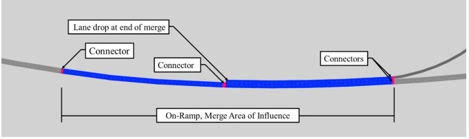
Figure 13-3: Freeway Merge Coding
The modeler typically uses the LCD of the connectors to accurately code the merge/weave area. One of the following two options can be implemented to avoid unrealistic lane changes on the freeway mainline into the acceleration lane:
- In the Connector dialog box, confirm the “Lane Change” distance for the connector downstream of the merge link is longer than the length of the merge area.
OR
- Indicate “No Lane Change” for the appropriate lane, using the Link dialog box.
13.4.4.2 Diverge
Freeway exit ramp diverge areas (parallel) are coded similar to the entrance ramp merge areas. The effective diverging area includes the entire auxiliary lane (or drop lane) starting at the taper and continuing to the painted gore point. The diverge section is typically one link with the number of lanes equal to the number of lanes on the freeway plus the number of lanes diverging from the freeway. There can only be one connector upstream of the diverge link. There can be two connectors downstream of the merge link, one for the ramp link and one for the main freeway link. The LCD can be coded similar to that of the merge/weave area of entrance ramps such that the distance exceeds that of the diverge area.
Freeway exit ramp diverge areas (taper) are coded using one connector placed at the painted gore point connecting the main freeway link to the ramp link. The main freeway link may not be broken with a connector. An appropriate LCD is recommended to be assigned to the connector to give vehicles enough time to merge to the correct lane to reach the exit ramp. A LCd is assigned such that it reflects the driver expectation and typically matches the location of the first guide or overhead sign indicating the approaching off-ramp. below illustrates a diverge segment.
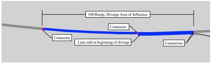
Figure 13-4: Freeway Diverge Coding
13.4.4.3 Weaving
Weave segments follow the same rules as merge and diverge areas. Appropriate LCD is assigned to connectors, so vehicles follow realistic weaving behavior. This can be based on guide sign placements or other driver behavior characteristics of the local area.
13.4.4.4 Managed Lanes
HOV managed lanes are coded by restricting certain vehicle classes from a lane in the link. It is best practice to code a separate HOV managed link display type to show which lane is coded as an HOV managed lane. These lanes can also be coded as an independent link if physically separated from the general-purpose lanes.
13.4.5 Basic Geometry – Arterial Coding
Intersections are coded using different links for each approach that end at the intersection. Links typically should not continue through the intersection and all movements for an intersection should be coded using connectors. For the introduction of additional lanes at intersection approaches, a separate link with the total number of intersection approach lanes is used downstream of the network link, using a single connector to smoothly make the transition. The link with the intersection approach lanes is typically the entire storage length of these lanes plus half the length of the taper for the developing lanes.
Once all approach links have been coded, connectors are used to code all possible movements at the intersection. The modeler typically follows the standard number of splines for each movement (if the standard number of splines does not accurately reflect the movement curvature, a different number of splines can be used):
- 12-point spline for left-turns;
- 8-point spline for right-turns;
- 15-spline for right-turn channelization; and
- 2-point spline for through movements
The modeler connects all connectors to the appropriate lane on the downstream link. For instance, connectors for right-turns connect to the right-most lane of the downstream link and connectors for left-turns to the left-most lane.
An RSA is coded on all turning movement connectors, so that vehicles slow their speed when making a turn. For right turns, 10 mph is typically used as the desired distribution for RSA. For left turns, 15 mph is typically used as the desired distribution for RSA.
13.4.5.1 Traffic Control Devices
Traffic control devices are an important part of network coding. There are numerous ways to code the different traffic control devices such as signalized intersections, AWSC intersections, two-way stop control (TWSC) intersections, roundabouts, etc. in Vissim. below provides a summary of the main network objects that are used to code the different types of traffic controls and their applications
Traffic Control | Description | Application |
|---|---|---|
Signal Heads | Signal heads are used to code signalized intersections and are assigned to the signal controller created for that intersection. Signal controllers are typically created using an *.RBC file that is imported from Synchro or created based on signal timing plans. |
|
Detectors | A detector is used to model traffic sensors in the field that help detect vehicles for actuated signal operations. |
|
Stop Signs | Stop signs are used to model unsignalized intersections. |
|
Conflict Rules | Conflict rules occur where two links or connectors overlap each other. They are initially set to a passive stage. If an actual conflict exists, the rules need to be adjusted to give one movement priority over the other based on the actual ROW for the conflict vehicles. |
|
Priority Rules | Priority rules are similar to conflict rules. They are used to model yield conditions, however, they allow for more customization and are recommended for use in complex situations. |
|
Roundabout | Roundabouts are typically coded using a combination of links, connectors, and priority rules/conflict areas. There are example demos within Vissim that can be used to understand the principles of coding a roundabout. |
|
13.4.5.2 Pedestrians
A pedestrian crosswalk is typically coded at an intersection using links that match the width and location of the crosswalk in the field that cross over the leg of the intersection. It is best practice to use a different display type for pedestrian crosswalk links to show that these are separate from the vehicle network links. Signal heads and detectors are used on the pedestrian crosswalk links for pedestrian movements controlled by a pedestrian signal. Conflict areas are coded between vehicle and pedestrian links. It is best practice to give priority to pedestrians by coding the green conflict area for pedestrian links and red for the overlapping vehicle links. However, conflict areas can lead to gridlock in certain situations, such as urban areas and areas with congestion. For those areas, it is recommended to use priority rules to avoid the network from gridlocking.
13.4.5.3 Transit
A transit route is coded to show where a transit vehicle moves within the model. These routes originate from the start of a link and are coded with a departure time, which determines the exact time the transit vehicle enters the network. Transit stops are coded along the network to provide locations where the transit vehicle stops. The duration of the stop is controlled using either a predetermined dwell time or passenger boarding. Dwell time distributions are used to code the predetermined dwell time.
Passenger boarding is coded by adding passengers in the network that board the transit vehicle at the stop. The modeler can toggle the transit stops as active/inactive for specific transit vehicles.
13.4.6 Network Loading
The next step in coding a Vissim model is adding vehicles, bicycles, and pedestrians to the network. For the purposes of this section, the word “vehicles” includes vehicles, bicycles, and pedestrians.
Vissim uses the European fleet as a default when beginning a new network. Change this setting to the American fleet to reflect longer vehicle lengths in America.
2D/3D models are the basis for the vehicle mix in the Vissim model. Each 2D/3D model is assigned a *.v3d model with a length of the vehicle that is simulated in the network. The distribution of the 2D/3D models is assigned using the 2D/3D model distributions, which establish the mix of 2D/3D models that appear in the network. The 2D/3D model distribution is assigned to the Vehicle Types. This provides a variety of vehicle lengths for each Vehicle Type used. For example, there can be several 2D/3D models that represent different models of cars. The 2D/3D distribution determines the ratio of each model of car expected to be seen in the network. The Vehicle Types for cars is assigned to this 2D/3D distribution so that the cars in the network show the correct ratio of each car model.
Vehicle Types are made of 2D/3D models. These aid in setting the variety of vehicles in the network. Vehicle Types are assigned to a specific Vehicle Composition that is used in a Vehicle Input to appear in the network.
Vehicle Compositions describe the type of vehicles simulated and are made of Vehicle Types. The Vehicle Composition is assigned to each individual vehicle input and determines the flow of different vehicle types. Vehicle Compositions typically have one or more Vehicle Type assigned to it. The Relative Flow determines what portion of the vehicle input volume is simulated as each Vehicle Type in the Vehicle Composition. For example, if a Vehicle Composition has three Vehicle Types with a total Relative Flow of 1 and a Relative Flow for Vehicle Type A of 0.25, then 25 percent of the vehicle input volume associated with that Vehicle Composition is simulated as Vehicle Type A.
Vehicle Classes are used to group Vehicle Types. Vehicle Classes typically contain any number of Vehicle Types, with the option to contain all Vehicle Types. Vehicle Classes provide the basis for speed data, evaluations, path selection behavior, and other network objects. For example, it is possible to restrict a Vehicle Class from entering a specific lane in a network link. The Vehicle Class does not determine the mix of vehicles in the network; this is determined by the Vehicle Composition.
Vehicle Inputs determine the volume of vehicles entering the network. These are assigned to specific links in units of vehicles per hour. Vehicle Inputs can either be stochastic (varies according to random functions based on the seed number for a given run) or exact (exact number of vehicles simulated as indicated by the flow rate). Microsimulation projects typically involve stochastic modeling of vehicle inputs. shows the relationship between the different network loading characteristics. Vehicle characteristics are shown in .
Characteristic | Summary |
|---|---|
Vehicle Type | Made of 2D/3D vehicle model distribution. |
Vehicle Composition | Made up of Vehicle Types. Vehicle composition is used to assign the percentage makeup of the traffic entering the network via Vehicle Inputs. |
Vehicle Class | Used to group Vehicle Types; can contain any number (or all) Vehicle Types |
Vehicle Input | Volume of vehicles entering the network; assigned to links in units of vehicles per hour. |
Vehicle Route | Determines where vehicles travel in a network. Most common route types are Static and Partial. |
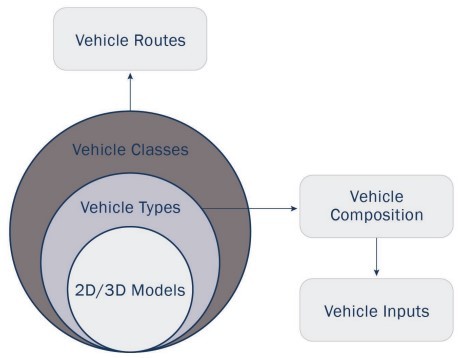
Figure 13-5: Relationship between the different network loading characteristics
Vehicle Routes are coded using Vehicle Routing Decisions and determine where the vehicles travel within the network. Relative Flows determine how many vehicles are assigned to each route based on the total number of vehicles that arrive at the Routing Decision during the time interval. There are many different types of Vehicle Routes, but the two most common are Static and Partial.
- Static Routes are used for base routing of network volumes. Static Routes are chosen to create relay routes that provide a new Routing Decision at each decision point. Static Routes can also be chosen to create end-to-end routes that account for travel patterns in the Vissim network and are often based on trip tables. Vehicle Routes default to the path of least resistance, but routes can be manually adjusted by the analyst. Static routes are typically used when no parallel routes exist in the model.
- Partial Routes are used for a secondary routing system of network volumes. Partial Routes can be used to control the Relative Flow of vehicles that are able to use multiple paths.
It is important to establish a consistent numbering scheme when coding Vehicle Inputs and Vehicle Routes. These numbering schemes are used when assigning inputs and routes at intersections.
DTA can be used in circumstances where parallel routes exist (i.e., multiple paths to and from an OD pair). Setting up a model with dynamic traffic assignment demand determining an OD matrix, coding nodes at the network corners, inserting nodes at diverging internal paths, and coding zones that are used as the origins and destinations. Using DTA can be a difficult and time-consuming process. It is recommended that DTA only be used if it is critical and cannot be substituted by static or partial routing.
13.4.7 Set up the Simulation and Run the Model
Before running a simulation, set up the desired Simulation Period, Random Seed Increment, and Number of Runs.
- The Simulation Period describes the total simulation time for each model run in simulation seconds.
- The Simulation Period is made up of the Seeding Period (time necessary for the network to become filled with vehicles) and Analysis Period (time that the network is evaluated for performance metrics).
- The Random Seed initializes a random number generator used to vary network conditions assigned using stochastic functions. This creates variations of behavior in the Vissim network that accounts for variations in real-world traffic conditions. The Random Seed Increment defines the difference between different Random Seeds of multiple simulation runs. It is best practice to keep the Random Seed Increment consistent between different models that are compared to one another in the same analysis.
- The Number of Runs determines the number of Random Seeds for the model to may run if the Random Seed Increment is greater than 0. Multiple model runs help account for variations in network operational performance. The variations between model runs result from variations in driver behavior in different Random Seeds. The Number of Runs are calculated based on the number of initial model runs, the mean and standard deviation of the initial run, t-statistic for the desired confidence level, and the tolerance error. More information is provided inSection 13.7.2.
Vissim begins each simulation without any vehicles in the model network, so some period of time is necessary to seed the network prior to collecting operational data. It is recommended that this Seeding Period (warmup period) be as long as necessary for the model to reach equilibrium. Equilibrium is reached when the number of vehicles entering the network is approximately equal to vehicles exiting the network. The number of vehicles entering and exiting the network are tracked during simulations to determine an appropriate initialization period. As discussed previously, the model simulation includes the build-up of congestion and the dissipation of congestion. Including this warmup and cool down period helps create a more accurate model.
13.4.8 Debugging
An important step after running a model is debugging. This is the process in which coding errors are identified and addressed. Coding within the network is typically checked so that it conforms to best practices and results in simulated conditions that are consistent with observed field conditions.
The debugging process is recommended to focus on checking the quality of big picture items such as the number of lanes, the RBCs used, and the location and type of DSD. The recommended method for debugging is to complete an initial review of the network prior to running the simulation, observe the model during the simulation, and/or review the error log file that may appear in a pop-up window. It is best practice to document the items checked while debugging.
Common coding errors are typically found in the following model objects:
- Signal timing/Signal Head assignments;
- Conflict Areas;
- DSD;
- Unusual vehicle behaviors due to errors in coding on network; and
- Types of Vehicle Inputs on Links
A checklist for debugging models is provided in
Appendix N, Section 1 – Model Debugging Checklist.