Section 3: Calibration Criteria Calculations Example
The first step to calibration is identifying a representative day from the cluster analysis. Cluster analysis is a statistical method that helps group (or cluster) data based on similarity between different parameters (travel time, throughput, weather, incidents, etc.). Each cluster represents a different set of travel conditions (weather-related, incident-related, normal, etc.) and will have a varying number of days associated with it. Multiple clusters that represent various driving scenarios may exist in the data set, depending on project scope, more than one cluster may be calibrated to and analyzed. Consult with the TxDOT project manager during scoping to determine the appropriate number of clusters to calibrate for.
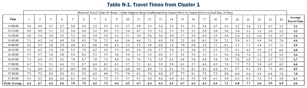
The example shown in this appendix shows the calculation from one travel condition and determines the representative day for that travel condition using one key measure and route, in this case, travel time in the southbound direction. However, to determine the representative day for a model, this calibration calculation should be done for a variety of key measures (travel time, speed, throughput, etc.) collected for all applicable routes and locations within the study area. below shows data from Cluster 1 of the cluster analysis. The table includes travel time from each day within the cluster and the analysis time period. shows a total of 24 days for the travel condition. However, it is important to note that the cluster analysis used to develop different travel conditions (weather-related, incident-related, normal, etc.) should be based on at least 100 days’ worth of data.
Below are the variables listed that are used across the different equations provided in the steps to calculate the representative day. The variables and equations are from FHWA’s Traffic Analysis Toolbox Volume III:
Guidelines for Applying Traffic Microsimulation Modeling Software 2019 Update
. The example and calculations have been modified to make it easier to follow the steps set out in the FHWA guidance.Step 1 – Calculate average travel time per time interval
Below is the equation for calculating the average for each 15-minute time interval across all days in the cluster.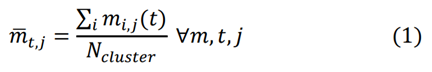
M | Set of measures of effectiveness considered for representative day |
m | Specific measure analyzed (travel time in this example) |
J | Set of routes and locations (only one route and location in this example) |
j | Specific route and location analyzed (only one route in this example) |
i | Observed day |
t | Time interval |
N cluster | Number of days in cluster |
Calculation results from equation (1) are shown in the last column of , which is the average travel time per time interval across all days in the cluster data set.
Step 2 – Calculate percentage difference between average value and observed value
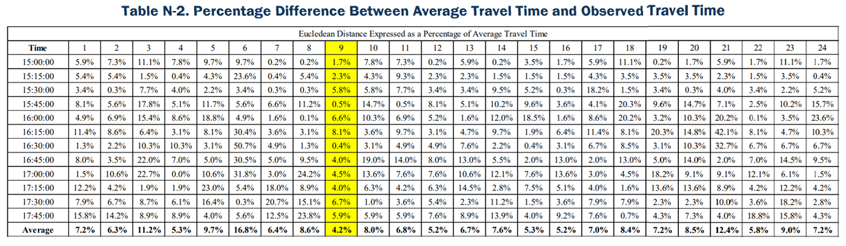
The next step is to calculate the percentage difference between average travel time for the time interval and the observed travel time for a particular day and the same time interval. This shown in equation (2) below.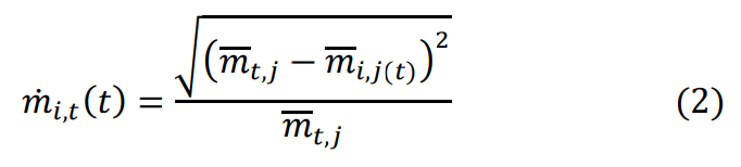
Below is an example of solving equation (2) for Day 1, Route 1, and the time interval 15:00:00.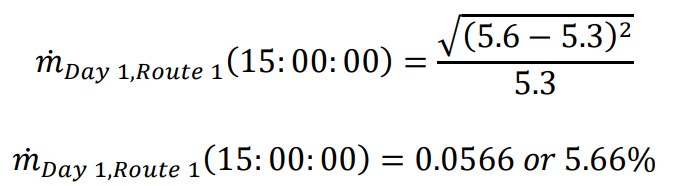
Step 3 – Calculate the average difference for each observed day and determine representative day
Determine the individual observed day that has the lowest average percentage. This can be done by averaging all routes, locations, and measures together for all the time intervals analyzed. Equation (3) below shows the formula to calculate this.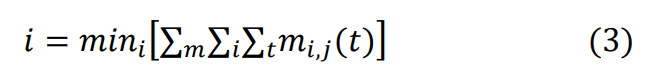
Because this example only uses one route and measure, only the travel time was averaged together for all time intervals for an observed day. If there were multiple routes, locations, and measures, all the different percentage differences calculated in Step 2 for the different measures, routes, and locations would be averaged together.
The last row in shows this calculation. As explained in Step 2, the percentages developed in were calculated by taking the absolute difference between the Average Travel Time (the last column in ) and the observed day travel time for the same time interval. In Step 3, these percentages are then averaged across all time intervals for the same day. The lowest average percentage is then considered the representative day. Day 9 had the lowest average at 4.2 percent; it is considered the representative day.
After determining the representative day, the analyst can start calibrating the model. The analyst will be calibrating against the measures used to determine representative day (travel time, in this example).
The 2019 FHWA guidance has four calibration criteria. Each criterion should be met for all the different measures, routes, and locations for the model to be considered calibrated. The variables and equations are from the FHWA 2019 guidance for microsimulation, but the example provided and calculations were modified to make it easier to follow the steps set out in the FHWA guidance.
Criterion I – Control for Time-Variant Outliers
Below is the summary of Criterion I, as well as an example.
Rationale and Criteria:
- Why: The purpose of this criteria is to control for maximum number of outliers associated with simulation results.
- Criteria: 95 percent of all simulated outputs should fall within the time-variant envelope created by the ~2 Sigma Band. Note that if fewer than 20-time intervals are used for the analysis, a maximum of one value may fall outside the time-variant envelope.
Variables and equations:
c r (t) | Observed travel times from the representative day |
σ(t) | Standard deviation for MOE for each time interval |
Z 95% | Z-Statistic for 95% of the observed variation |
Equations for calculating ~2 Sigma Band:
~2 Sigma Band Maximum Value: 𝐼̂ ~2 (𝑡) = c + r (t)Z 95% (σ(t)) | (4) |
~2 Sigma Band Maximum Value: 𝐼̂ ~2 (𝑡) = c - r (t)Z 95% (σ(t)) | (5) |
Example calculation
Step 1 – Calculate the standard deviation per time interval.
To calculate the standard deviation, the analyst must use the values from . Below is the equation for standard deviation of a population. Note that the FHWA guidance uses a standard deviation of a population equation and not for a sample.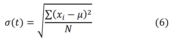
Where,
σ(t) | population standard deviation per time interval |
x i | each value from the population (observed travel time) |
µ | the population mean (average travel time from last column in ) |
N | size of the population (total number of days in cluster) |
A sample calculation for standard deviation for one time interval is provided below.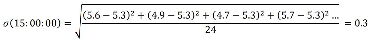
This calculation is repeated for each time interval. Results can be found in the third column of .
Step 2 – Calculate ~ 2 sigma band max and min for each time interval
Equations (4) and (5) above can be used to calculate the ~2 Sigma Bands. The Z95% statistic is provided in the FHWA guidance and is 1.96. An example calculation for the 15:00:00 time interval for these equations is shown below. The standard deviation calculated in the previous step is used for the ~2 sigma band calculations.
~2 Sigma Band Maximum Value: 𝐼̂
~2
(15:00: 00) = 5.2 + 1.96(0.3) = 5.9 min
~2 Sigma Band Minimum Value: 𝐼̂
~2
(15:00: 00) = 5.2 - 1.96(0.3) = 4.5 min
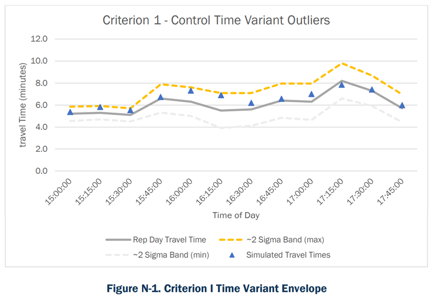
Columns four and five in below show the results of the ~2 sigma band calculations for all the time intervals. The variation envelope developed using the ~2 sigma band is shown in .
Time of Trip Start | Rep. Day Travel Time | Standard Deviation | ~2 Sigma Band (max) | ~2 Sigma Band (min) | Simulated Travel Times | Simulated Value Within ~2 Sigma Band? |
15:00:00 | 5.2 | 0.3 | 5.9 | 4.5 | 5.4 | YES |
15:15:00 | 5.3 | 0.3 | 5.9 | 4.7 | 5.8 | YES |
15:30:00 | 5.1 | 0.3 | 5.7 | 4.5 | 5.5 | YES |
15:45:00 | 6.6 | 0.7 | 7.9 | 5.3 | 6.7 | YES |
16:00:00 | 6.3 | 0.7 | 7.6 | 5.0 | 7.3 | YES |
16:15:00 | 5.5 | 0.8 | 7.1 | 3.9 | 6.9 | YES |
16:30:00 | 5.6 | 0.8 | 7.1 | 4.1 | 6.2 | YES |
16:45:00 | 6.4 | 0.8 | 8.0 | 4.8 | 6.6 | YES |
17:00:00 | 6.3 | 0.8 | 7.9 | 4.7 | 7.0 | YES |
17:15:00 | 8.2 | 0.8 | 9.8 | 6.6 | 7.8 | YES |
17:30:00 | 7.3 | 0.7 | 8.7 | 5.9 | 7.4 | YES |
17:45:00 | 5.7 | 0.6 | 7.0 | 4.4 | 6.0 | YES |
As seen in the above, all the simulated travel times for the different time intervals fall within the time variant envelopes created by the ~2 sigma band. Because there are fewer than 20 time-intervals, the FHWA criterion allows one simulated travel time to fall outside of the ~2 sigma band. Based on the calculations, Criterion I is satisfied.
Criterion II – Control for Time-Variant “Inliers”
Below is the summary of Criterion II, as well as an example.
Rationale and Criteria:
- Why: The purpose of this criteria is to constrain simulated results to fall closely in line with the representative day.
- Criteria: 2/3 of all simulated outputs and simulated results for 2 critical time intervals must fall within the time-variant envelope created by the ~1 Sigma Band. Note that the two critical time intervals must be non-adjacent maximum values from the representative day.
Variables and equations:
c r (t) | Observed travel times from the representative day |
σ(t) | Standard deviation for MOE for each time interval |
Equations for calculating ~2 Sigma Band:
1 Sigma Band Maximum Value: 𝐼̂ 1 (𝑡) = 𝑐𝑟 (𝑡) + 𝜎(𝑡) | (6) |
1 Sigma Band Maximum Value: 𝐼̂ 1 (𝑡) = 𝑐𝑟 (𝑡) - 𝜎(𝑡) | (7) |
Example calculation
Step 1 – Calculate 1 sigma band maximum and minimum values.
Because standard deviation was already calculated as part of Criterion I, there is no need to calculate it again. Below is an example calculation for equations (6) and (7).
1 Sigma Band Maximum Value: 𝐼̂ 1 (15: 00: 00) = 5.2 + 0.3 = 5.5 min | |
1 Sigma Band Maximum Value: 𝐼̂ 1 (15: 00: 00) = 5.2 - 0.3 = 4.9 min |
Columns four and five in below show the results of the 1 sigma band calculations for all time intervals. The variation envelope developed using the 1 sigma band is shown in .
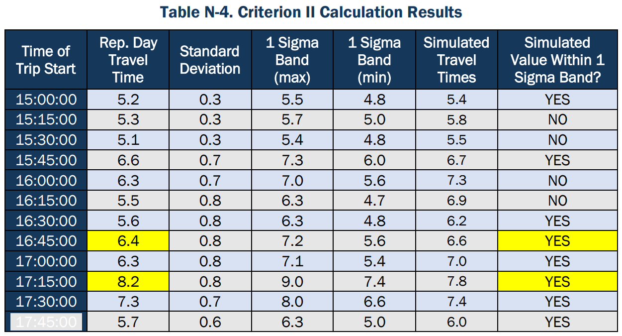
As seen in above, eight out of the 12 simulated travel times fall within the 1 sigma band time-variant envelope. The criterion calls for 2/3 of all simulated results to fall within the 1 sigma band, which is satisfied.
The second part of this criterion calls for two non-consecutive critical outputs to also fall within the 1 sigma band. The critical outputs are determined by two maximum non-consecutive travel times from the representative day. The first critical output to check the simulated travel time against is at 17:15:00 time interval, when the representative day travel time is at the highest, 8.2 minutes. The second critical output occurs at 17:30:00 time interval, when the representative day travel time is at 7.3 minutes. However, this value cannot be used because it is adjacent to the first critical value. The next critical output occurs at 15:45:00, when the representative day travel time is 6.6 minutes. The simulated travel time at 17:15:00 and at 15:45:00 falls within the 1 sigma band.

Criterion III – Bounded Dynamic Absolute Error (BDAE)
Below is the summary of Criterion III, as well as an example.
Rationale and Criteria:
- Why: To determine on average, the simulated results are close to the representative day.
- Criteria: Average simulated absolute error from the representative day overall time intervals is less than or equal to the BDAE. The BDAE is the differences from the representative day seen across all days in the cluster for all time intervals.
Variables and equations:
c r (t) | Observed value of representative day during time interval t |
c i (t) | Observed value of non-representative day within the cluster during time interval t |
𝑐̃ r (t) | Simulated performance measure during time interval t |
N T | Number of time intervals |
N cluster | Number of days in the cluster representing travel condition |
BDAE threshold equation: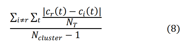
Average simulated absolute error equation: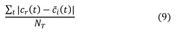
Criterion III is met when: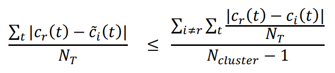
Or in other words, Criterion III is met when the average simulated absolute error is less than or equal to the BDAE threshold.
Example Calculation
Step 1 – Calculate the average simulated absolute error.
To calculate average simulated absolute error, take the absolute value between the difference of the simulated travel time and the representative day travel time for each time interval, sum all the absolute value differences together for all time intervals, and divide by the total number of time intervals. This calculation is provided below; results are shown in .
Below is the calculation for the average simulated absolute error from equation (9).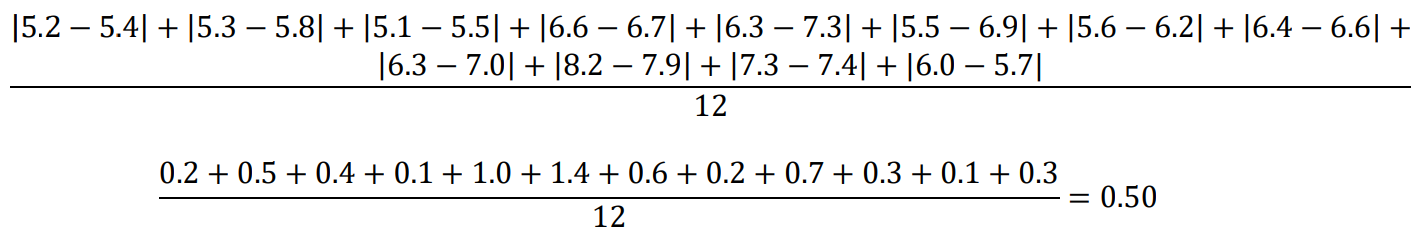
The average simulated absolute error is equal to 0.5.
Time of Trip Start | Simulated Travel Time | Rep. Day Travel Time | Absolute Difference |
15:00:00 | 5.4 | 5.2 | 0.2 |
15:15:00 | 5.8 | 5.3 | 0.5 |
15:30:00 | 5.5 | 5.1 | 0.4 |
15:45:00 | 6.7 | 6.6 | 0.1 |
16:00:00 | 7.3 | 6.3 | 1.0 |
16:15:00 | 6.9 | 5.5 | 1.4 |
16:30:00 | 6.2 | 5.6 | 0.6 |
16:45:00 | 6.6 | 6.4 | 0.2 |
17:00:00 | 7.0 | 6.3 | 0.7 |
17:15:00 | 7.9 | 8.2 | 0.3 |
17:30:00 | 7.4 | 7.3 | 0.1 |
17:45:00 | 6.0 | 5.7 | 0.3 |
Average | 0.5 | ||
Step 2 – Calculate the BDAE threshold
The BDAE is a more involved calculation but can be done easily with a spreadsheet program such as Microsoft Excel. The first part of the calculation is to take the absolute difference between the representative day and the observed day within the cluster and divide by the total number of time intervals. This is then done for all the days that do not equal the representative day and all-time intervals within the cluster. This part of the calculation is shown below.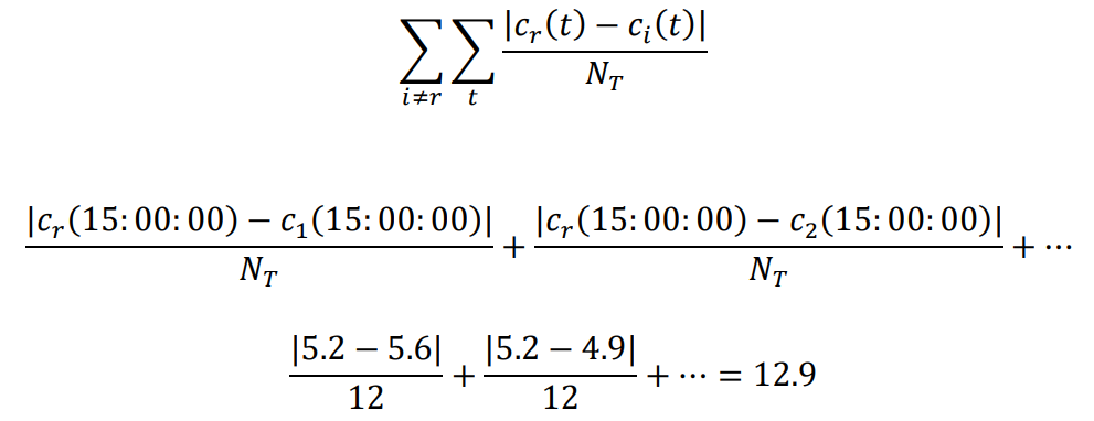
The next part of the calculation is to divide this result by the number of days in the cluster minus 1.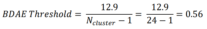
Criterion III is met when the average simulated absolute error is less than or equal to the BDAE threshold: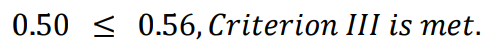
Criterion IV – Bounded Dynamic Systematic Error
Below is the summary of Criterion IV, as well as an example.
Rationale and Criteria:
- Why: To ensure the simulation is not over- or under-estimating the representative day.
- Criteria: Average simulated error from the representative day over all time intervals is less than or equal to 1/3 the BDAE.
Variables and equations:
c r (t) | Observed value of representative day during time interval t |
c i (t) | Observed value of non-representative day within the cluster during time interval t |
𝑐̃ r (t) | Simulated performance measure during time interval t |
N T | Number of time intervals |
N cluster | Number of days in the cluster representing travel condition |
Average simulated absolute error equation: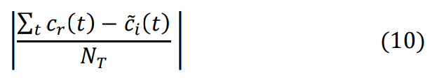
The dissimilarity between equation (9) and equation (10) is that the absolute value in equation (10) is taken after averaging the differences together, whereas in equation (9) the absolute value is taken after the difference and those values are summed together, and then the average is taken. Below is the calculation for the average simulated error from equation (10).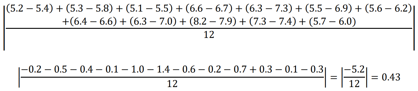
Criterion IV is met when the average simulated error is less than or equal to the 1/3 BDAE threshold: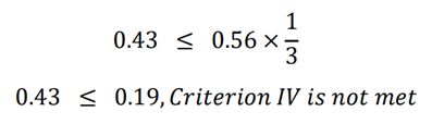
Criterion IV is not met, and the simulation is an overestimation of the representative day travel time. The analyst would have to go back to the microsimulation software and modify parameters to make the travel time more closely match with the representative day.