5.3.4 HSM Part C – Predictive Method
Part C of the HSM provides a predictive method to estimate average crash frequencies for both existing and proposed future conditions of a roadway network, facility, or individual site. This predictive method not only estimates total crashes over a given time but can also be used to estimate average crash frequencies by crash severity and collision type. It is recommended that these estimates be determined for existing conditions, alternatives to the existing conditions, or for proposed new roadways. A roadway network can be divided into individual sites of either homogenous roadway segments or intersections to run the predictive method.
The estimated average crash frequency of an individual facility type is based on the traffic volumes, geometric design features, and traffic control type for that site. Predictive models were developed to estimate average crash frequencies for a variety of facility types using regression models. These regression models were developed from data of similar sites across the country and are known as safety performance functions (SPFs) in the HSM. SPFs have been developed for specific facility types under what are referred to as “base conditions,” the most common conditions for similar sites across the country. For
example
, shows a sample of the base conditions for rural multilane highways.Undivided Roadways | Divided Roadways | Intersections |
|---|---|---|
Lane width: 12 feet | Lane width: 12 feet | Intersection skew angle: 0 degrees |
Shoulder width: 6 feet | Right shoulder width: 8 feet | No intersection left-turn lanes except on stop-controlled approaches |
Shoulder type: Paved | Median width: 30 feet | No intersection right-turn lanes except on stop-controlled approaches |
No lighting | No lighting | No lighting |
The HSM has developed the SPFs for the following facility types:
- Rural two-lane, two-way roads;
- Rural multilane highways;
- Urban and suburban arterials; and
- Freeways and ramps (2014 supplement)
Facility Type | Undivided Roadway Segment | Divided Roadway Segment | Intersections | |||
|---|---|---|---|---|---|---|
Stop Control on Minor Leg(s) | Signalized | |||||
3-Leg | 4-Leg | 3-Leg | 4-Leg | |||
Rural Two-Lane, Two-Way Road | ✓ | ✓ | ✓ | ✓ | ||
Rural Multilane Highways | ✓ | ✓ | ✓ | ✓ | ✓ | |
Urban and Suburban Arterials | ✓ | ✓ | ✓ | ✓ | ✓ | ✓ |
Facility Type | Classification | Rural | Urban |
|---|---|---|---|
Freeway Segment | Four-Lane | ✓ | ✓ |
Six-Lane | ✓ | ✓ | |
Eight-Lane | ✓ | ✓ | |
Ten-Lane | ✓ | ||
Ramp Segments | One-Lane Entrance Ramp | ✓ | ✓ |
One-Lane Exit Ramp | ✓ | ✓ | |
Two-Lane Entrance Ramp | ✓ | ||
Two-Lane Exit Ramp | ✓ | ||
Collector-Distributor Road (C-D) | One-Lane C-D Road | ✓ | ✓ |
Two-Lane C-D Road | ✓ | ||
Ramp Terminal | One-Way Stop-Controlled Two-, Three-, or Four-Lane Crossroad | ✓ | ✓ |
Signalized Two-Lane Crossroad | ✓ | ✓ | |
Signalized Three-Lane Crossroad | ✓ | ✓ | |
Signalized Four-Lane Crossroad | ✓ | ✓ | |
Signalized Five-Lane Crossroad | ✓ | ||
Signalized Six-Lane Crossroad | ✓ |
A simplified
example
of how SPFs were developed for the HSM is illustrated in . This figure illustrates how crash data from across the country was used in the development of the SPFs located in the HSM.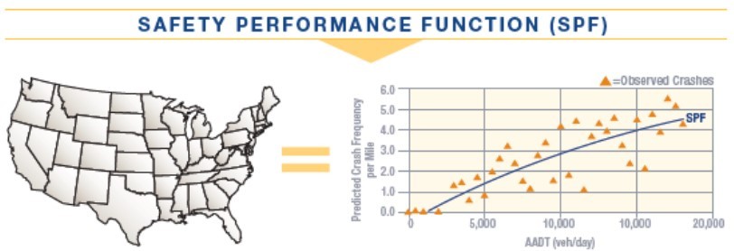
Figure 5-3: Example SPF Development
Adjustments to the predicted crashes, determined by using an SPF, may account for the differences between the base conditions used in developing the SPF and the site-specific conditions.
Part C CMFs are used to account for these differences when site-specific conditions vary from the base conditions. These CMFs were developed specifically for individual SPFs and are intended to be applied only to the crash prediction results of that particular SPF. The SPF-related CMFs are different than the CMFs on the CMF Clearinghouse website. The Highway Safety Manual 2nd Edition (HSM2) is expected to rename SPF-related CMFs to AFs to reduce the confusion between Part C CMFs developed for a specific SPF and CMFs located on the Clearinghouse website.
A calibration factor (C) may also be used to make agency-specific adjustments to the predicted crash totals. This accounts for the differences between the agency or agencies for which the models were developed and the agency/agencies for which the predictive model is being applied. Calibration factors to the HSM predictive method calculations should be applied whenever possible. Each agency is responsible for developing their own calibration factors for specific facility types.
The HSM Part C predictive method is summarized in the following general equation:
N
Predicted
= NSPFX
× (CMF1x
× CMF2x
× ... × CMFnx
) × Cx
Where:
N
= predicted average crash frequency for a specific site typePredicted
N
= predicted average crash frequency for the base conditions of the SPF for a specific site typeSPFX
CMF
= CMF specific to the SPF for a specific site type1x
C
= calibration factor to adjust the specific SPF to the local conditions for a specific site typex
x
= specific site typeBecause crash totals fluctuate over time, it is difficult to know whether changes in the observed crash totals are due to changes in site conditions or are due to natural fluctuations. A period with a high number of observed crashes is statistically likely to be followed by a period with a low number of observed crashes. The opposite of this tendency also applies; it is probable that a period with low crash totals will be followed by a period with high crash totals. This tendency to regress to the mean or average is known as regression-to-the-mean (RTM). Failure to account for the effects of RTM introduces the potential for RTM bias, also known as selection bias. RTM bias results in overestimating or underestimating the effectiveness of a treatment. The effects of RTM bias are illustrated in . For existing sites, facilities, or roadways, the Empirical Bayes (EB) method can be applied within the predictive method to account for both the predicted average crash frequency and the observed crash frequency. This method accounts for the reliability of a particular SPF and RTM bias.
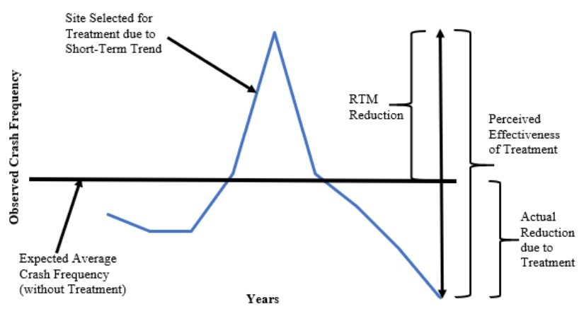
Figure 5-4: Regression to Mean Bias
The application of the EB method within the predictive method results in an expected average crash frequency. illustrates the relationship between observed, predicted, and expected crashes when performing the predictive method for a particular SPF. See
Appendix F, Section 2 – NCHRP 17-50 Project Example of HSM in Design
for more details on how expected crashes can be estimated.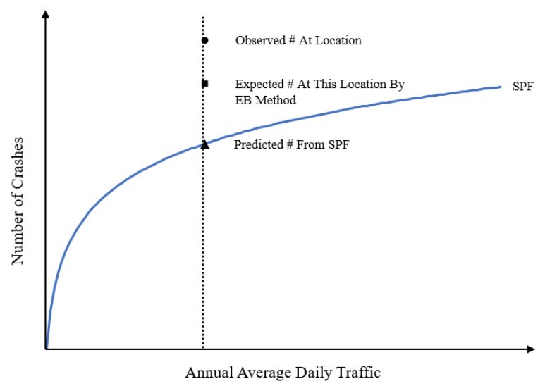
Figure 5-5: Relationship of Observed, Predicted, and Expected Crashes within the Predictive Method
identifies the scenarios when the EB method is applicable and not applicable, as identified in the HSM.
EB Method is Not Applicable (Predicted Crashes) | EB Method is Applicable (Expected Crashes) |
EB method is not applicable for the following types of situations:
| EB method is applicable for the following situations:
|
The HSM predictive method is summarized as an 18-step process used to estimate average crash frequencies for a roadway network, facility, or site and is illustrated in . An example of applying the HSM Part C predictive method is provided in
Appendix F, Section 2 – NCHRP 17-50 Project Example of HSM in Design
.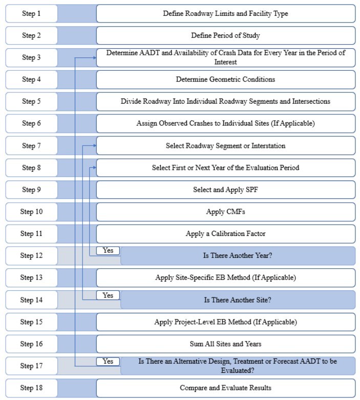
Figure 5-6: HSM Predictive Method 18-Step Process