Log-Pearson Type III Distribution Fitting Procedure
The log-Pearson type III (LPIII) statistical distribution method is recommended in
and is the standard of practice for estimating annual probability of exceedance of peak flows. An outline of this method follows. However, the designer is not limited to using this method, especially if the resulting flow-frequency relation does not seem to fit the data.
The following general procedure is used for LPIII analyses.
The LPIII, Skew, and Accommodation of Outliers procedures described below are still based on information from Bulletin #17B. The latest HDM update occurred soon after the release of #17C and during ongoing TxDOT research on updating skew procedures. Recent edits in this section simply introduce Bulletin #17C. A future HDM version will update these sections to reflect latest #17C procedures. Meanwhile, refer to Bulletin #17C
for further information.- Acquire and assess the annual peak discharge record.
- Compute the base 10 logarithm of each discharge value.
- Compute the mean, standard deviation, and (station) of the log flow values.
- Compute the weighted skew coefficient from the station skew and regional skew.
- Identify high and low from the sample set.
- Recompute the mean, standard deviation, and station skew of the log flow values with outliers removed from the sample set.
- Compute flow values for desired AEPs.
With the LPIII method, the logarithm of the discharge for any AEP is calculated as:
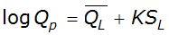
Equation 4-2.
Where:
 = mean of the logarithms of the annual peak discharges
- Qp= flood magnitude (cfs or m3/s) of AEP p
- K= frequency factor for AEP p and coefficient of skew appropriate for site
- S= standard of deviation of logarithms of the annual peak dischargesL
See the spreadsheet
for values of K, based on station skew coefficient.
The three statistical moments used to describe the LPIII distribution are the mean, standard deviation, and skew. Estimates of these moments for the distribution of the entire population of flows are computed for the available sample of flows with the equations below.
The mean is given by:
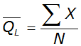
Equation 4-3.
Where:
- = mean of the (base 10) logarithms of the annual peak discharges
- X= logarithm of the annual peak discharge
- N= number of observations
The standard deviation is given by:
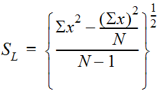
Equation 4-4.
Where:
- S= standard deviation of the logarithms of the annual peak discharge; N and X are defined as aboveL
The coefficient of skew (station skew) is given by:
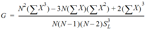
Equation 4-5.
Where:
- G= coefficient of skew of log values; N, X, and SLare defined as above
Skew represents the degree of curvature to the flow-frequency curve as shown in Figure 4-3. In Figure 4-3 the X-axis scale is probability (symmetric at about AEP = 0.5) and the Y-axis scale is base 10 logarithmic flow. A skew of zero results in a straight-line flow frequency curve. A negative skew value produces a flow-frequency curve with lesser flows than the zero skew line, and a positive skew produces a flow-frequency curve with greater flows than the zero skew line.
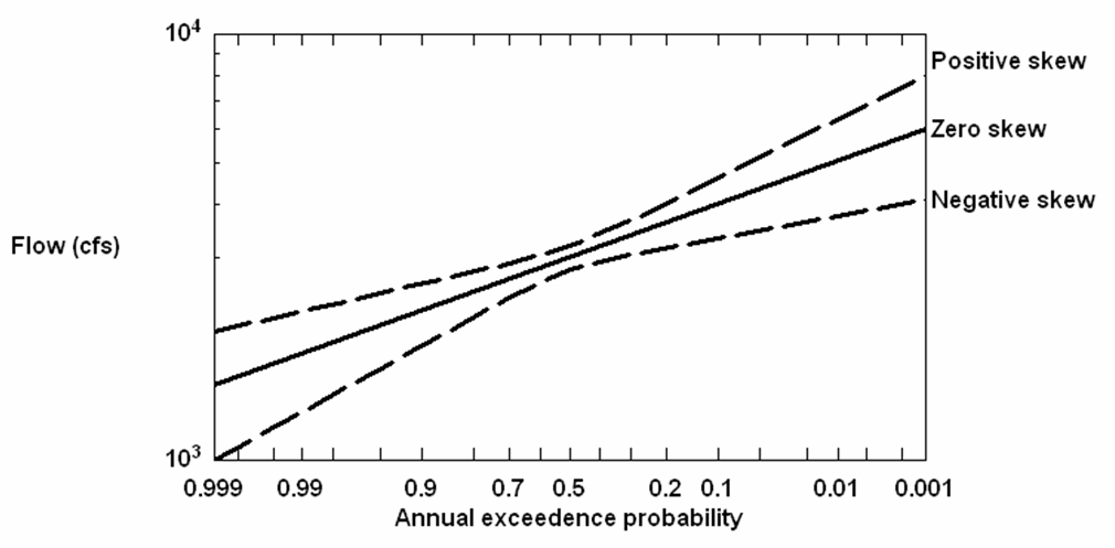
Figure 4-3. Skew of discharge versus frequency plots
The following cases require special consideration.
provides further guidance:
- Record is incomplete—flows missing from record becausethey weretoo small or too large to measure (flows filtered from record based on flow magnitude).
- Record contains zero flow values—stream was dry all year.
- Record contains historical flows not recorded in a systematic fashion. Examples are extreme events recorded prior to or after installation of a stream gauge. These are indicated by code in USGS annual .
- Flows are the result of two distinct types (a mixed population) of hydrologic events such as snowmelt and rainstorms.