Selecting a Sea Level Rise Value for Design
Relative sea level rise should be incorporated in project design if project is characterized as having:
|
When incorporating relative sea level rise into project design, it is important to select a future sea level rise projection that considers the project design life and risk tolerance to flooding. Climate change modeling and sea level rise projections have continued to evolve with significant advances in the understanding of global and regional factors that contribute to relative sea level rise. In 2019, the Texas General Land Office (GLO) published an updated
(GLO Plan), which includes detailed relative sea level rise scenarios for the state. The GLO Plan relies on the global sea level rise projections released in the 2017 NOAA report
, which reflects the latest published and peer-reviewed sea level science. The 2017 NOAA report includes six global sea level rise scenarios (low, intermediate low, intermediate, intermediate high, high, and extreme) to examine the full range of potential future water levels.
The 2017 NOAA projections have the added advantage of providing risk-based (probabilistic) planning capabilities, which were not previously available. The range of probabilities for each planning timeframe is dependent on modeled future climate conditions (referred to as Representative Concentration Pathways – or RCP), as described in the Intergovernmental Panel on Climate Change (IPCC)
(AR5).
To address the impacts of relative sea level rise during the next 50 to 100 years, the GLO Plan adjusted NOAA’s intermediate scenario of a 3.3-foot global mean sea level increase by 2100 to account for local effects (e.g., vertical land movement, tectonics, and sediment compaction) through statistical analysis of local tide stations along the Texas coast. This intermediate scenario has a 2 to 17 percent chance of being exceeded by future global sea levels by the year 2100. These local effects are what differentiate sea level rise from relative sea level rise and account for the relative portion of the rates.
Because of the diversity and expanse of the Texas coastline, the GLO Plan divides the coastal area into four regions to provide a more focused assessment within each region (Figure 15-11). The regions contain unique environmental characteristics, land use patterns, and vertical land movement that affect local water levels. Table 15-6 provides average relative sea level rise projections for each region. When considering future conditions for project design, a regional projection representative of the project location should be selected.
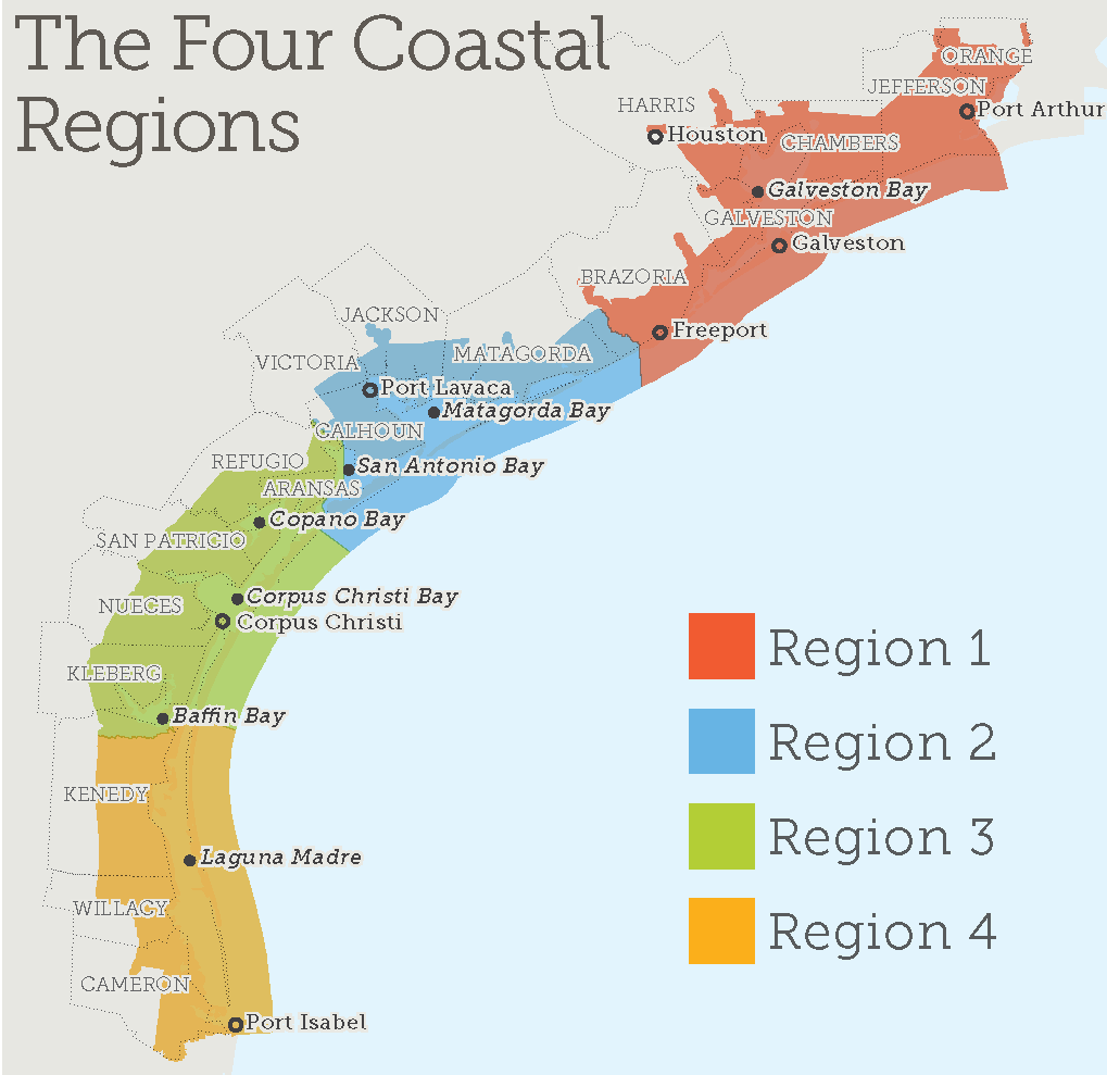
Figure 15-11. The GLO Texas Coastal Resiliency Master Plan’s Four Coastal Regions (Texas General Land Office, 2019).
Planning Time Horizon | Relative Sea Level Rise (feet) | |||
|---|---|---|---|---|
(Year) | Region 1 | Region 2 | Region 3 | Region 4 |
2020 | 0.8 | 0.8 | 0.7 | 0.6 |
2030 | 1.3 | 1.2 | 1.1 | 1.0 |
2040 | 1.7 | 1.6 | 1.5 | 1.3 |
2050 | 2.2 | 2.1 | 1.9 | 1.7 |
2060 | 2.8 | 2.6 | 2.4 | 2.2 |
2070 | 3.4 | 3.2 | 3.0 | 2.8 |
2080 | 4.1 | 3.9 | 3.6 | 3.3 |
2090 | 4.8 | 4.6 | 4.3 | 4.0 |
2100 | 5.5 | 5.2 | 5.0 | 4.6 |
Notes:
| ||||
The design life of transportation infrastructure describes the time period the structure is expected to sustain usability under normal loads and conditions and varies depending on the particular asset type. TxDOT refers to the American Association of State Highway and Transportation Officials (AASHTO) Bridge Design Specifications for bridge design life, and bridges are typically designed considering a 75-year period. Roadways are typically designed considering a 50-year period. In both instances, the relative sea level rise over the lifespan of the asset may be significant and should be considered in the design. Quantifying relative sea level rise into the project design will be dependent on the design life.
For example, if a project takes place in Region 1 and entails the installation of flexible pavement with a design life of 20 years starting in the year 2020, 0.9 feet of relative sea level rise is recommended in the design. This is calculated by subtracting 0.8 feet of relative sea level rise (year 2020) from 1.7 feet of relative sea level rise (year 2040) to account for the relative sea level rise that is expected to occur since the start of the project.
To consider a more complex example, consider a project in Region 2 starting in 2025 that will install concrete pavement roadway, which has a 30-year design life, connecting to a bridge, which has a 75-year design life. The relative sea level rise projection used for the road would be 1.4 feet (2.4 feet [year 2055] minus 1.0 feet [year 2025]). The relative sea level rise projection for the bridge would be 4.2 feet (5.2 feet [year 2100] minus 1.0 feet [year 2025]). The designer will need to consider whether elevating the roadway to the elevation of the bridge is feasible and appropriate for the project to conserve the life of the bridge asset.
To allow incremental adjustments to manage the impacts of relative sea level rise, the design of some transportation assets (e.g., causeway heights, pavement surfaces, facility protection design, and roadside vegetation) could also target a shorter intended design life. For example, a causeway could consider a 30-year design life rather than a 75-year design life so that future climate conditions are more moderate and achievable based on project cost restrictions and efficiencies. The
Consideration of Sea Level Rise in Project Design
section below describes additional criteria to consider when incorporating relative sea level rise into transportation projects.In Summer 2019, FHWA is expected to release an update to their Hydraulic Engineering Circular 25 (HEC-25)
report. The updated edition will include recommendations for incorporating sea level rise into project design and should be reviewed prior to development of stillwater levels.
Considering Relative Sea Level Rise in Project Design
Once projections for relative sea level rise have been identified for the project, the following procedures should be followed:
- Obtain elevation data for project site features (e.g., roadway, culvert, bridge). Project elevations can be obtained from as-built drawings for maintenance projects or from land surveys completed for planned projects.
- Select a relative sea level rise projection from Table 15-6 based on the appropriate region to assess potential impacts.
- Using the project survey elevation data collected in step 1 and relative sea level projections from step 2, assess the relative sea level rise over the project lifespan.
- If applicable, identify the possible negative impacts of relative sea level rise on the project related to asset function or operation. Possible impacts include scour and/or erosion due to tidal action, reduced efficiency of drainage culverts due to higher tailwater conditions, and exposure to saltwater.
- For identified impacts, assess if adaptive measures will be necessary. In many cases, the project footprint may be impacted, but no adaptive measures may be required. Impacts may also be temporary (e.g., wave splash during high tide events or during storms). Not all adaptive measures require physical alteration to the roadway design. Temporary impacts may be addressed through operational modifications, such as short-term road closures.
- Identify the cost of potential relative sea level rise adaptive measures. Due to cost limitations, not all relative sea level rise adaptive measures may be included in the project design. For example, raising a roadway could cause a larger fill slope to encroach into an environmentally sensitive area. Assessments of potential adaptation measures and any limitations should be documented to indicate what can be achieved through evaluating the cost of adaptation vs. the cost of inaction. Costs should be considered in terms of economic, environmental, and social/human impacts.
- Where feasible, adaptive measures for relative sea level rise (e.g., roads elevated on berms, bridge height and on ramp adjusted for future sea levels, long-term planned retreat, enhanced erosion protection along roadway) should be incorporated into project design, particularly where future impacts are anticipated.
- Consider unintended hydraulic impacts when designing relative sea level rise adaptive measures. For example, elevating roadways may impede floodwater drainage or affect flooding of adjacent properties. To offset these impacts, incorporating additional drainage mechanisms into project design can alleviate flooding of low-lying areas located near the modified roadway.
Sea Level Rise Projection Sources
- Texas General Land Office— 2019 Texas Coastal Resiliency Master Plan, published February 28, 2019.
- FHWA— Highways in the Coastal Environment: Volume 3, anticipated publish date in Summer 2019
- NOAA– Global and Regional Sea Level Rise Scenarios for the United States, published January 2017. e 2017 NOAA report
Selecting Stillwater Levels for Project Design
Selecting appropriate stillwater levels for each project is critical for transportation infrastructure located in coastal areas. Stillwater levels are used as input for the design wave height (Section 3), which when combined, determine the design elevation. This cumulative elevation is discussed further in Section 4 of this chapter. The stillwater level at a project site is composed of a combination of the appropriate astronomical tide and storm surge, as previously discussed. If sea level rise is to be accounted for, it will be cumulatively combined with the tidal information.
Stillwater level is a combination of:
|
While the 1% AEP storm tide is the primary flood zone mapped by FEMA as either AE or VE zones, coastal transportation projects (e.g., local roadway) frequently justify a lower AEP (e.g., 50% to 10% AEP) and others (e.g., freeways or critical evacuation routes) that may justify a higher exceedance probability (e.g., 2% or 1% AEP). Knowing when, where, and how to appropriately select and apply a stillwater level comes from experience and sound judgement. Refer to Chapter 4 (Hydrology), Section 6 (Design Flood and Check Flood Standards) as a starting point for consideration by roadway classification and structure type. As demonstrated in this section, this decision is dependent on numerous factors and can be a subjective process unique to the coastal zone. Proficiencies in this topic typically reside with the Precertified Coastal Engineer; however, it is important that the designer demonstrate knowledge and competence assessing the project risk tolerance, budget restraints, and social and environmental impacts to select the most appropriate stillwater level for a safe, yet cost-effective project design.
For a project relying on a Level 1 or 2 analysis (e.g., local roads/street or other non-critical assets), it may be acceptable to develop a stillwater elevation by adding an appropriate sea level rise projection, as determined by the project’s design life and risk tolerance, to a FEMA return period storm tide collected from the latest FIS for the project area (after excluding wave heights).
More complex projects that require a Level 3 analysis are likely to require additional effort. To obtain a site-specific water elevation needed for design, the designer may need to work with a Precertified Coastal Engineer to perform risk-based modeling of water level conditions that capture the local variability experienced at the project site. These models will simulate a number of possible independent storm scenarios that include a variety of storm parameters, including wind speed, pressure, and landfall angle, among others, combined with statistical analysis to determine the probability of the storm tide occurring at the project site. These models will also be capable of incorporating changes in relative sea level to evaluate how the return period design events chosen may evolve over time. Some descriptions of how these models are developed and utilized are described in subsequent sections.